2. Essence 1. Choice of the time interval for imaging

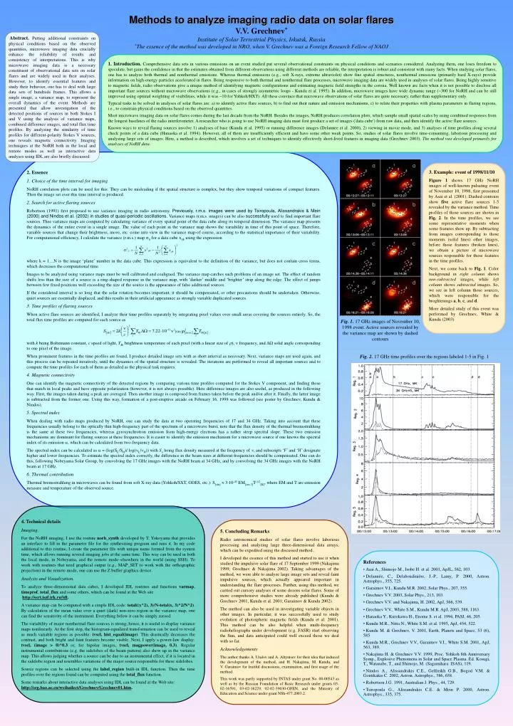
1. 2. Essence 1. Choice of the time interval for imaging NoRH correlation plots can be used for this. They can be misleading if the spatial structure is complex, but they show temporal variations of compact features. Then the image set over this time interval is produced. 2. Search for active flaring sources Robertson(1991) first proposed to use variance imaging in radio astronomy. Previously, r.m.s. images were used by Tsiropoula, Alissandrakis & Mein (2000) and Nindos et al. (2002) in studies of quasi-periodic oscillations. Variance maps (r.m.s. images) can be also successfully used to find important flare sources. Thee variance maps are computed by calculating variance of every spatial point of the data cube along its temporal dimension. The variance map presents the dynamics of the entire event in a single image. The value of each point in the variance map shows the variability in time of this point of space. Therefore, variable sources that change their brightness, move, etc. come into view in the variance map-of course, according to the statistical importance of their variability. For computational efficiency, I calculate the variance (r.m.s.) map ij for a data cube xijk using the expression where k = 1…N is the image ‘plane’ number in the data cube. This expression is equivalent to the definition of the variance, but does not contain cross terms, which decreases the computational time. Images to be analyzed using variance maps must be well calibrated and coaligned. The variance map catches such problems of an image set. The effect of random shifts less than the size of a source is a ring-shaped response in the variance map, with ‘darker’ middle and ‘brighter’ strip along the edge. The effect of jumps between few fixed positions well exceeding the size of the source is the appearance of false additional sources. If the considered interval is so long that the solar rotation becomes important, it should be compensated, or other precautions should be undertaken. Otherwise, quiet sources are essentially displaced, and this results in their artificial appearance as strongly variable duplicated sources. 3. Time profiles of flaring sources When active flare sources are identified, I analyze their time profiles separately by integrating pixel values over small areas covering the sources entirely. So, the total flux time profiles are computed for each source as with k being Boltzmann constant, c speed of light, TBi brightness temperature of each pixel (with a linear size of ),  frequency, and  solid angle corresponding to one pixel of the image. When prominent features in the time profiles are found, I produce detailed image sets with as short interval as necessary. Next, variance maps are used again, and this process can be repeated iteratively, until the dynamics of the spatial structure is revealed. The iterations are performed to reveal all important sources and to compute the time profiles for each of them as detailed as the physical task requires. 4. Magnetic connectivity One can identify the magnetic connectivity of the detected regions by comparing various time profiles computed for the Stokes V component, and finding those that match in local peaks and have opposite polarization (however, it is not always possible). Here difference images are also useful, as produced in the following way. First, the images taken during a peak are averaged. Then another image is composed from frames taken before the peak and/or after it. Finally, the latter image is subtracted from the former one. Using this way, formation of a post-eruptive arcade on February 16, 1999 was followed (see poster by Grechnev, Kundu & Nindos). 5. Spectral index When dealing with radio maps produced by NoRH, one can study the data at two operating frequencies of 17 and 34 GHz. Taking into account that these frequencies usually belong to the optically thin high-frequency part of the spectrum of a microwave burst, note that the flux density of the thermal bremsstrahlung is the same at these two frequencies, whereas gyrosynchrotron emission from high-energy electrons has a rather steep spectral slope. These two emission mechanisms are dominant for flaring sources at these frequencies. It is easier to identify the emission mechanism for a microwave source if one knows the spectral index of its emission , which can be calculated from two-frequency data. The spectral index can be calculated as  = (log(SL/SH)/ log(L/H)) with S being flux density measured at the frequency of , and subscripts ‘F’ and ‘H’ designate higher and lower frequencies. To estimate the spectral index correctly, the difference in the beam sizes at different frequencies should be compensated. One can do this, following Nobeyama Solar Group, by convolving the 17 GHz images with the NoRH beam at 34 GHz, and by convolving the 34 GHz images with the NoRH beam at 17 GHz. 6. Thermal contribution Thermal bremsstrahlung in microwaves can be found from soft X-ray data (Yohkoh/SXT, GOES, etc.): S[sfu] 310-45 EM[cm-3]T-1/2[K], where EM and T are emission measure and temperature of the observed source. Fig. 1. 17 GHz images of November 10, 1998 event. Active sources revealed by the variance map are shown by dashed contours Fig. 2. 17 GHz time profiles over the regions labeled 1-5 in Fig. 1 Methods to analyze imaging radio data on solar flaresV.V. Grechnev*Institute of Solar Terrestrial Physics, Irkutsk, Russia*The essence of the method was developed in NRO, when V. Grechnev was a Foreign Research Fellow of NAOJ Abstract.Putting additional constraints on physical conditions based on the observed quantities, microwave imaging data crucially enhance the reliability of results and consistency of interpretations. This is why microwave imaging data is a necessary constituent of observational data sets on solar flares and are widely used in their analyses. However, to identify essential features and study their behavior, one has to deal with large data sets of hundreds frames. This allows a single image, a variance map, to represent the overall dynamics of the event. Methods are presented that allow investigation of the detected positions of sources in both Stokes I and V using the analysis of variance maps, combined difference images, and total flux time profiles. By analyzing the similarity of time profiles for different-polarity Stokes V sources, one reveals magnetic connectivity. Imaging techniques at the NoRH both in the local and remote modes as well as interactive data analyses using IDL are also briefly discussed. 1. Introduction.Comprehensive data sets in various emissions on an event studied put several observational constraints on physical conditions and scenarios considered. Analyzing them, one loses freedom to speculate, but gains the confidence in that the estimates obtained from different observations using different methods are reliable, the interpretation is robust and consistent with many facts. When studying solar flares, one has to analyze both thermal and nonthermal emissions. Whereas thermal emissions (e.g., soft X-rays, extreme ultraviolet) show fine spatial structures, nonthermal emissions (primarily hard X-rays) provide information on high-energy particles accelerated in flares. Being responsive to both thermal and nonthermal flare processes, microwave imaging data are widely used in analyses of solar flares. Being highly sensitive to magnetic fields, radio observations give a unique method of identifying magnetic configurations and estimating magnetic field strengths in the corona. Well known are facts when it is not possible to disclose all important flare sources without microwave observations (e.g., in cases of strongly asymmetric loops - Kundu et al. 1995). In addition, microwave images have wide dynamic range (~300 for NoRH and can be still improved using optimal weighting of visibilities, while it was ~10 for Yohkoh/HXT). All these convince that microwave observations of solar flares are quite necessary, rather than supplementary only. Typical tasks to be solved in analyses of solar flares are: a) to identify active flare sources, b) to find out their nature and emission mechanisms, c) to relate their properties with plasma parameters in flaring regions, i.e., to constrain physical conditions based on the observed quantities. Mozt microwave imaging data on solar flares comes during the last decade from the NoRH. Besides the images, NoRH produces correlation plots, which sample small spatial scales by using combined responses from the longest baselines of the radio interferometer. A researcher who is going to use NoRH imaging data must first produce a set of images ('data cube') from raw data, and then identify the active flare sources. Known ways to reveal flaring sources involve 1) analyses of base (Kundu et al. 1995) or running difference images (Delannee et al. 2000), 2) viewing in movie mode, and 3) analyses of time profiles along several check points of a data cube (Hanaoka et al. 1994). However, all of them are insufficiently efficient and have some other weak points. So, studies of solar flares involve time-consuming, laborious processing and analyzing large sets of images. Here, a method is described, which involves a set of techniques to identify effectively short-lived features in imaging data (Grechnev 2003). The method was developed primarily for analyses of NoRH data. 3. Example: event of 1998/11/10 Figure 1 shows 17 GHz NoRH images of well-known pulsating event of November 10, 1998, first presented by Asai et al. (2001). Dashed contours show five active flare sources 1-5 revealed by the variance method. Time profiles of those sources are shown in Fig. 2. In the time profiles, we see some representative moments when some features show up. By subtracting from images corresponding to those moments (solid lines) other images, before those features (broken lines), we obtain a picture of microwave sources responsible for those features in the time profiles. Next, we come back to Fig. 1. Color background in right column shows non-subtracted images, while left column shows subtracted images. So, we see in left column those sources, which were responsible for the broghtenings a, b, c, and d. More detailed study of this event was performed by Grechnev, White & Kundu (2003) 4. Technical details Imaging. For the NoRH imaging, I use the routine norh_synth developed by T. Yokoyama that provides an interface to fill in the parameter file for the synthesizing program and runs it. In my code additional to this routine, I create the parameter file with unique name formed from the system time, which allows running several imaging jobs at the same time. This way can be used in both the local mode, in Nobeyama, and the remote mode–elsewhere in the world (using SSH). To work with routines that need graphical output (e.g., MAP_SET to work with the orthographic projection) in the remote mode, one can use the Z buffer graphics device. Analysis and Visualization. To analyze three-dimensional data cubes, I developed IDL routines and functions varmap, timeprof, total_flux and some others, which can be found at the Web site http://ssrt.iszf.irk.ru/idl. A variance map can be computed with a simple IDL code: total((x^2), 3)/N-total(x, 3)^2/N^2). By calculation of the mean value over a quiet (dark) non-zero region in the variance map, one can find the sensitivity of the instrument. Everything below it can be simply zeroed. The variability of major nonthermal flare sources is strong; hence, it is useful to display variance maps nonlinearly. At the first step, the histogram-equalized transformation can be used to reveal as much variable regions as possible: tvscl, hist_equal(image). This drastically decreases the contrast, and both bright and faint features become visible. Next, I apply a power-law display: tvscl, (image > 0)^0.3 or, for bipolar images, tvscl, magpower(image, 0.3). Regular instrumental contributions (e.g. the sidelobes of the beam pattern) also show up in the variance map. This allows judging whether a source can be due to an instrumental effect, if it is located in the sidelobe region and resembles variations of the major source responsible for these sidelobes. Source regions can be selected using the label_region built-in IDL function. Then the time profiles over the regions found can be computed using the total_flux function. Some remarks about interactive data analyses using IDL can be found at the Web site: http://srg.bao.ac.cn/weihailect/Grechnev/Grechnev01.htm. 5. Concluding Remarks Radio astronomical studies of solar flares involve laborious processing and analyzing large three-dimensional data arrays, which can be expedited using the discussed method.. I developed the essence of this method and started to use it when studied the impulsive solar flare of 17 September 1999 (Nakajima 1999; Grechnev & Nakajima 2002). Taking advantages of the method, we were able to analyze large image sets and reveal faint impulsive sources, which actually appeared important in understanding the flare processes. Further, using this method, we carried out cursory analyses of some dozens solar flares. Some of more comprehensive studies were already published (Kundu & Grechnev 2001, Kundu et al. 2001; Garaimov & Kundu 2002). The method can also be used in investigating variable objects in other images. In particular, it was successfully used to study evolution of photospheric magnetic fields (Kundu et al. 2001). This method can be also helpful when multi-frequency radioheliographs under development (e.g. FASR) start observing the Sun, and data anticipated could well exceed those we deal with so far. Acknowledgements The author thanks A. Uralov and A. Altyntsev for their idea that induced the development of the method, and H. Nakajima, M. Kundu, and V. Garaimov for fruitful discussions, examination, and first usage of the method. This work was partly supported by INTAS under grant No. 00-00543 as well as by the Russian Foundation of Basic Research under grants 03-02-16591, 03-02-16229, 02-02-39030-GFEN, and the Ministry of Education and Science under grant NSh-477.2003.2. • References • Asai A., Shimojo M., Isobe H. et al. 2001, ApJL, 562, 103. • Delannée, C., Delaboudinière, J.-P., Lamy, P. 2000, Astron. Astrophys., 355, 725. • Garaimov V.I., Kundu M.R. 2002, Solar Phys., 207, 355. • Grechnev V.V. 2003, Solar Phys., 213, 103. • Grechnev V.V. and Nakajima, H. 2002, ApJ, 566, 539. • Grechnev V.V., White S.M., Kundu M.R. ApJ, 2003, 588, 1163. • Hanaoka Y., Kurokawa H., Enome S. et al. 1994, PASJ, 46, 205. • Kundu M.R., Nitta N., White S.M. et al. 1995, ApJ, 454, 522. • Kundu M. & Grechnev, V. 2001, Earth, Planets and Space, 53 (6), 585 • Kundu M.R., Grechnev V.V., Garaimov V.I., White S.M. 2001, ApJ, 563, 389. • Nakajima H. & Grechnev V.V. 1999, Proc. Yohkoh 8th Anniversary Symp., Explosive Phenomena in Solar and Space Plasma. Ed. Kosugi, T., Watanabe, T., and Shimojo, M. (Sagamihara: ISAS), 119. • Nindos A., Alissandrakis C.E., Gelfreikh G.B., Bogod V.M. & Gontikakis C. 2002, Astron. Astrophys., 386, 658. • Robertson J.G. 1991, Australian J. Phys., 44, 729. • Tsiropoula G., Alissandrakis C.E. & Mein P. 2000, Astron. Astrophys., 335, 375.