Download

1 / 48
490 likes | 579 Views
Discover the first success story of DNA sequence comparison in bioinformatics, uncovering gene similarities and functions through dynamic programming techniques. Explore how this approach helped find the gene responsible for cystic fibrosis and how dynamic programming was used to solve the Manhattan Tourist Problem. Learn about the pitfalls of greedy algorithms and recursive programs compared to dynamic programming. Through examples and explanations, grasp the essence of finding optimal paths and scores in weighted grids using dynamic programming.

E N D
Dynamic Programming: Sequence alignment CS 466 Saurabh Sinha
DNA Sequence Comparison: First Success Story • Finding sequence similarities with genes of known function is a common approach to infer a newly sequenced gene’s function • In 1984 Russell Doolittle and colleagues found similarities between cancer-causing gene and normal growth factor (PDGF) gene • A normal growth gene switched on at the wrong time causes cancer !
Cystic fibrosis (CF) is a chronic and frequently fatal genetic disease of the body's mucus glands. CF primarily affects the respiratory systems in children. Search for the CF gene was narrowed to ~1 Mbp, and the region was sequenced. Scanned a database for matches to known genes. A segment in this region matched the gene for some ATP binding protein(s). These proteins are part of the ion transport channel, and CF involves sweat secretions with abnormal sodium content! Cystic Fibrosis
Role for Bioinformatics • Gene similarities between two genes with known and unknown function alert biologists to some possibilities • Computing a similarity score between two genes tells how likely it is that they have similar functions • Dynamic programming is a technique for revealing similarities between genes
Dynamic programming example:Manhattan Tourist Problem Imagine seeking a path (from source to sink) to travel (only eastward and southward) with the most number of attractions (*) in the Manhattan grid Source * * * * * * * * * * * * Sink
Dynamic programming example:Manhattan Tourist Problem Imagine seeking a path (from source to sink) to travel (only eastward and southward) with the most number of attractions (*) in the Manhattan grid Source * * * * * * * * * * * * Sink
Manhattan Tourist Problem: Formulation Goal: Find the longest path in a weighted grid. Input: A weighted grid G with two distinct vertices, one labeled “source” and the other labeled “sink” Output: A longest path in Gfrom “source” to “sink”
MTP: An Example 0 1 2 3 4 j coordinate source 3 2 4 0 3 5 9 0 0 1 0 4 3 2 2 3 2 4 13 1 1 6 5 4 2 0 7 3 4 15 19 2 i coordinate 4 5 2 4 1 0 2 3 3 3 20 3 8 5 6 5 2 sink 1 3 2 23 4
22 MTP: Greedy Algorithm Is Not Optimal 1 2 5 source 3 10 5 5 2 5 1 3 5 3 1 4 2 3 promising start, but leads to bad choices! 5 0 2 0 0 0 0 sink 18
MTP: Simple Recursive Program MT(n,m) ifn=0 or m=0 returnMT(n,m) x MT(n-1,m)+ length of the edge from (n- 1,m) to (n,m) y MT(n,m-1)+ length of the edge from (n,m-1) to (n,m) returnmax{x,y} What’s wrong with this approach?
Here’s what’s wrong • M(n,m) needs M(n, m-1) and M(n-1, m) • Both of these need M(n-1, m-1) • So M(n-1, m-1) will be computed at least twice • Dynamic programming: the same idea as this recursive algorithm, but keep all intermediate results in a table and reuse
MTP: Dynamic Programming j 0 1 source 1 0 1 S0,1= 1 i 5 1 5 S1,0= 5 • Calculate optimal path score for each vertex in the graph • Each vertex’s score is the maximum of the prior vertices score plus the weight of the respective edge in between
MTP: Dynamic Programming (cont’d) j 0 1 2 source 1 2 0 1 3 S0,2 = 3 i 5 3 -5 1 5 4 S1,1= 4 3 2 8 S2,0 = 8
MTP: Dynamic Programming (cont’d) j 0 1 2 3 source 1 2 5 0 1 3 8 S3,0 = 8 i 5 3 10 -5 1 1 5 4 13 S1,2 = 13 5 3 -5 2 8 9 S2,1 = 9 0 3 8 S3,0 = 8
MTP: Dynamic Programming (cont’d) j 0 1 2 3 source 1 2 5 0 1 3 8 i 5 3 10 -5 -5 1 -5 1 5 4 13 8 S1,3 = 8 5 3 -3 3 -5 2 8 9 12 S2,2 = 12 0 0 0 3 8 9 S3,1 = 9 greedy alg. fails!
MTP: Dynamic Programming (cont’d) j 0 1 2 3 source 1 2 5 0 1 3 8 i 5 3 10 -5 -5 1 -5 1 5 4 13 8 5 3 -3 2 3 3 -5 2 8 9 12 15 S2,3 = 15 0 0 -5 0 0 3 8 9 9 S3,2 = 9
MTP: Dynamic Programming (cont’d) j 0 1 2 3 source 1 2 5 0 1 3 8 Done! i 5 3 10 -5 -5 1 -5 1 5 4 13 8 (showing all back-traces) 5 3 -3 2 3 3 -5 2 8 9 12 15 0 0 -5 1 0 0 0 3 8 9 9 16 S3,3 = 16
si-1, j + weight of the edge between (i-1, j) and (i, j) si, j-1 + weight of the edge between (i, j-1) and (i, j) max si, j = MTP: Recurrence Computing the score for a point (i,j) by the recurrence relation: The running time is n x m for a n by mgrid (n = # of rows, m = # of columns)
A2 A3 A1 B sA1 + weight of the edge (A1, B) sA2 + weight of the edge (A2, B) sA3 + weight of the edge (A3, B) max of sB = Manhattan Is Not A Perfect Grid What about diagonals? • The score at point B is given by:
max of sy + weight of vertex (y, x) where y є Predecessors(x) sx = Manhattan Is Not A Perfect Grid (cont’d) Computing the score for point x is given by the recurrence relation: • Predecessors (x) – set of vertices that have edges leading to x • The running time for a graph G(V, E) (V is the set of all vertices and Eis the set of all edges) is O(E) since each edge is evaluated once
Traveling in the Grid • By the time the vertex x is analyzed, the values sy for all its predecessors y should be computed – otherwise we are in trouble. • We need to traverse the vertices in some order • For a grid, can traverse vertices row by row, column by column, or diagonal by diagonal
Traversing the Manhattan Grid a) b) • 3 different strategies: • a) Column by column • b) Row by row • c) Along diagonals c)
Traversing a DAG • A numbering of vertices of the graph is called topological ordering of the DAG if every edge of the DAG connects a vertex with a smaller label to a vertex with a larger label • How to obtain a topological ordering ?
matches mismatches insertions deletions 4 1 2 match 2 mismatch deletion indels insertion Aligning DNA Sequences Alignment : 2 x k matrix ( km, n ) n = 8 V = ATCTGATG m = 7 W = TGCATAC V W
Longest Common Subsequence (LCS) – Alignment without Mismatches • Given two sequences • v = v1v2…vm and w = w1w2…wn • The LCS of vand w is a sequence of positions in • v: 1 < i1 < i2 < … < it< m • and a sequence of positions in • w: 1 < j1 < j2 < … < jt< n • such that it -th letter of v equals to jt-letter of wand t is maximal
0 1 2 2 3 3 4 5 6 7 8 0 0 1 2 3 4 5 5 6 6 7 LCS: Example i coords: elements of v A T -- C -- T G A T C elements of w -- T G C A T -- A -- C j coords: (0,0) (1,0) (2,1) (2,2) (3,3) (3,4) (4,5) (5,5) (6,6) (7,6) (8,7) positions in v: 2 < 3 < 4 < 6 < 8 Matches shown inred positions in w: 1 < 3 < 5 < 6 < 7 Every common subsequence is a path in 2-D grid
si-1, j si, j-1 si-1, j-1 + 1 if vi = wj max si, j = Computing LCS Let vi = prefix of v of length i: v1 … vi and wj = prefix of w of length j: w1 … wj The length of LCS(vi,wj) is computed by:
LCS Problem as Manhattan Tourist Problem A T C T G A T C j 0 1 2 3 4 5 6 7 8 i 0 T 1 G 2 C 3 A 4 T 5 A 6 C 7
Edit Graph for LCS Problem A T C T G A T C j 0 1 2 3 4 5 6 7 8 i 0 T 1 G 2 C 3 A 4 T 5 A 6 C 7
Edit Graph for LCS Problem A T C T G A T C j 0 1 2 3 4 5 6 7 8 Every path is a common subsequence. Every diagonal edge adds an extra element to common subsequence LCS Problem: Find a path with maximum number of diagonal edges i 0 T 1 G 2 C 3 A 4 T 5 A 6 C 7
Backtracking • si,j allows us to compute the length of LCS for vi and wj • sm,n gives us the length of the LCS for v and w • How do we print the actual LCS ? • At each step, we chose an optimal decision si,j = max (…) • Record which of the choices was made in order to obtain this max
si-1, j si, j-1 si-1, j-1 + 1 if vi = wj max si, j = Computing LCS Let vi = prefix of v of length i: v1 … vi and wj = prefix of w of length j: w1 … wj The length of LCS(vi,wj) is computed by:
Printing LCS: Backtracking • PrintLCS(b,v,i,j) • if i = 0 or j = 0 • return • ifbi,j = “ “ • PrintLCS(b,v,i-1,j-1) • printvi • else • ifbi,j = “ “ • PrintLCS(b,v,i-1,j) • else • PrintLCS(b,v,i,j-1)
From LCS to Alignment • The Longest Common Subsequence problem—the simplest form of sequence alignment – allows only insertions and deletions (no mismatches). • In the LCS Problem, we scored 1 for matches and 0 for indels • Consider penalizing indels and mismatches with negative scores • Simplest scoring scheme: +1 : match premium -μ : mismatch penalty -σ : indel penalty
Simple Scoring • When mismatches are penalized by –μ, indels are penalized by –σ, and matches are rewarded with +1, the resulting score is: #matches – μ(#mismatches) – σ (#indels)
The Global Alignment Problem Find the best alignment between two strings under a given scoring schema Input : Strings v and w and a scoring schema Output : Alignment of maximum score → = -σ = 1 if match = -µ if mismatch si-1,j-1 +1 if vi = wj si,j = max s i-1,j-1 -µ if vi ≠ wj s i-1,j - σ s i,j-1 - σ m : mismatch penalty σ : indel penalty {
Scoring Matrices To generalize scoring, consider a (4+1) x(4+1) scoring matrixδ. In the case of an amino acid sequence alignment, the scoring matrix would be a (20+1)x(20+1) size. The addition of 1 is to include the score for comparison of a gap character “-”. This will simplify the algorithm as follows: si-1,j-1 + δ(vi, wj) si,j = max s i-1,j + δ(vi, -) s i,j-1 + δ(-, wj) {
Making a Scoring Matrix • Scoring matrices are created based on biological evidence. • Alignments can be thought of as two sequences that differ due to mutations. • Some of these mutations have little effect on the protein’s function, therefore some penalties, δ(vi , wj), will be less harsh than others.
AKRANR KAAANK -1 + (-1) + (-2) + 5 + 7 + 3 = 11 Scoring Matrix: Example • Notice that although R and K are different amino acids, they have a positive score. • Why? They are both positively charged amino acids will not greatly change function of protein.
Conservation • Amino acid changes that tend to preserve the physico-chemical properties of the original residue • Polar to polar • aspartate glutamate • Nonpolar to nonpolar • alanine valine • Similarly behaving residues • leucine to isoleucine
Local vs. Global Alignment • The Global Alignment Problem tries to find the longest path between vertices (0,0) and (n,m) in the edit graph. • The Local Alignment Problem tries to find the longest path among paths between arbitrary vertices (i,j) and (i’, j’) in the edit graph. • In the edit graph with negatively-scored edges, Local Alignment may score higher than Global Alignment
Compute a “mini” Global Alignment to get Local Alignment Local Alignment: Example Local alignment Global alignment
Local Alignments: Why? • Two genes in different species may be similar over short conserved regions and dissimilar over remaining regions. • Example: • Homeobox genes have a short region called the homeodomain that is highly conserved between species. • A global alignment would not find the homeodomain because it would try to align the ENTIRE sequence
The Local Alignment Problem • Goal: Find the best local alignment between two strings • Input : Strings v, w and scoring matrix δ • Output : Alignment of substrings of v and w whose alignment score is maximum among all possible alignment of all possible substrings
The Problem Is … • Long run time O(n4): - In the grid of size n x n there are ~n2 vertices (i,j) that may serve as a source. - For each such vertex computing alignments from (i,j) to (i’,j’) takes O(n2) time. • This can be remedied by allowing every point to be the starting point
Notice there is only this change from the original recurrence of a Global Alignment The Local Alignment Recurrence • The largest value of si,j over the whole edit graph is the score of the best local alignment. • The recurrence: 0 si,j = max si-1,j-1 + δ(vi, wj) s i-1,j + δ(vi, -) s i,j-1 + δ(-, wj) {