Download

1 / 33
330 likes | 431 Views
Analyzing sorting algorithms. Recall that T(n) represents the time required for an algorithm to process input of size n. For a sorting algorithm, T(n) represents the time needed to sort. this time may be the worst-case time, the average-case time, or something else.

E N D
Analyzing sorting algorithms • Recall that T(n) represents the time required for an algorithm to process input of size n. • For a sorting algorithm, T(n) represents the time needed to sort. • this time may be the worst-case time, the average-case time, or something else
Comparison-based sorting algorithms • Many sorting algorithms are comparison based – they depend on being able to compare pairs of elements. • this constraint is naturally represented in Java by the Comparable and Comparator interfaces • In this case we often let T(n) be the number of element comparisons.
Divide-and-conquer sorting algorithms • For divide-and-conquer, we define T(n) in terms of the value of T on smaller arguments. • For example, selection sort applies divide-and-conquer to the output, as follows: • find a piece of size 1 of the output sequence (find the smallest item; swap it with the first item) • sort the remaining n-1 elements • Here T(n) = n-1 + T(n-1), where T(1) = 0 • since the first phase uses n-1 comparisons, and the second phase takes time T(n-1)
Insertion sort • The insertion sort algorithm has the following form: • insert a piece of size 1 (usually, the last element) • into the result of sorting a piece of size n-1 • We get the same constraint as above for T(n) • if T(n) is interpreted as the worst-case number of comparisons • note that this worst case can be achieved
Time complexity of insertion sort and selection sort • We need to solve the recurrence relation T(n) = n-1 + T(n-1); T(1) = 0 • But this is the relation that describes the sum of the first n nonnegative integers • cf. the first S expression on p.5 of Weiss • but with index bounds 0 and n-1 • So T(n) = (n-1)n/2 • And selection sort is Q(n2) • And insertion sort is Q(n2) in theworst case
Sorting algorithms we’ve seen • Binary search tree (BST) sort • insert all items into a BST, and traverse • time complexity is Q(n2) in the worst case • and Q(n log n) in the best case • Heapsort • build a heap, then delete all items • building a heap takes time Q(n) • deletions take time Q(n log n) in the worst case • so sorting also has worst-case time Q(n log n)
Other divide-and-conquer sorting algorithms • Mergesort: • sort two pieces of size n/2 • merge the sorted pieces • Quicksort constructs the output in a divide-and-conquer way: • preprocess the input so that small items are to the left and large items are to the right • sort both pieces
Nonrecursive sorting algorithms • Insertion sort, selection sort, and mergesort are easy to formulate nonrecursively. • Quicksort can be formulated recursively by using an explicit stack • some optimization is possible by doing so.
Bottom-up mergesort • Mergesort is easy to state in a bottom-up manner. • Initial sorted subsequences (runs) may be created in any convenient manner • or may simply be taken to be sequences of size 1 • A single pass merges pairs of adjacent runs into larger runs
Space use in mergesort • Top-down: all recursive calls can share the same temporary array • those subarrays that overlap in time don’t overlap in space • In the bottom-up version, passes may copy data alternately into and out of a temporary array • an extra pass may be needed to get output into the desired array
Time complexity of mergesort • The bottom-up version has Q(log n) passes • each pass requires time Q(n) • so the overall time complexity is Q(n log n) • The relevant recursion is T(n) = 2T(n/2) + cn • and has solution T(n) = Q(n log n) • For both top down and bottom up, data flow may be modeled by a binary merge tree • in each case the merge tree has height Q(log n) • and each level takes time Q(n) to process
Merge tree (bottom up, n = 19) XXXXXXXXXXXXXXXXXXX / \ XXXXXXXXXXXXXXXX XXX / \ | XXXXXXXX XXXXXXXX XXX / \ / \ | XXXX XXXX XXXX XXXX XXX /\ /\ /\ /\ / \ XX XX XX XX XX XX XX XX XX X
Merge tree (top down, n = 19) XXXXXXXXXXXXXXXXXXX / \ XXXXXXXXX XXXXXXXXXX / \ / \ XXXX XXXXX XXXXX XXXXX / \ / \ / \ / \ XX XX XX XXX XX XXX XX XXX XX / \ / \ / \ X XX X XX X XX
Quicksort • Recall that for quicksort, a preprocessing step is needed • to get small elements to the left of the array • and large elements to the right of the array • A partition function performs this step • The partition function compares each array element to a pivot element. • pivot elements usually come from the input array • if so, partition can put them between the small and large items
Quicksort details • Small input needn’t be sorted recursively • another sorting algorithm can be used • “small” means of size less than about 10 or 20 • The partition function typically works by using two index variables i and j • i starts at the left and moves right • it looks for large values to move right • j starts at the right and moves left • it looks for small values to move left
More quicksort details • After i and j have both stopped moving • the items pointed to by i and j are swapped unless they have crossed • If i and j have not crossed • then they both start moving again • else neither moves again • The partition function takes linear time • since moving i and j toward one another one step takes time O(1)
Partitioning issues in quicksort Issues for partition: • how to choose the pivot • the pivot element should be unlikely to be large or small (even for nonrandom input) • how to initialize i and j • what if i or j finds a copy of the pivot? • why don’t i and j pass the end of the array? • at the end, where does the pivot element go?
Weiss suggests: • letting the pivot be the median of the left, center, and right elements • sorting these three values in place • initially swapping the pivot with the element in position right-1
Other suggestions from Weiss • i & j should be advanced first -- then referenced • so i should start at left and j at right-1 • When either i or j sees the pivot element, it should stop • Explicit tests shouldn’t be needed to keep i and j from running off the end of the array • instead, sentinels should be available • At the end, the pivot element should be swapped into position i
Informal analysis of quicksort • In the best case of quicksort, partitioning always splits the input sequence evenly • so we get the recurrence of mergesort • and thus time complexity Q(n log n) • In the worst case, partitioning leaves n-b elements in the big piece, for a fixed bound b • so T(n) = T(n-b) + p(n) • where p(n), the time to partition, is Q(n) • as for insertion & selection sort, this gives a time complexity of Q(n2)
The selection problem • The selection problem is to find the kth smallest element an unsorted collection. • One way to select is to sort first • in time Q(n log n) • Faster ways are possible
Selection using quicksort • A selection algorithm based on quicksort is available • with average case time complexity Q(n log n) • Here we partition as before • Based on how the parameter k compares to the final index of the pivot we may determine • which half the kth item will be in, and • a new parameter for recursively sorting this half
Bucket sort and radix sort • There's an important family of sorting algorithms that don’t depend on comparing pairs of elements • If the elements being sorted needn't all be distinct, these algorithms can run in time faster than n log n
Conditions for bucket sort • Bucket sort can be used when there is a function f that assigns indices to input elements so that if A <= B, f(A) <= f(B). • Here f is similar to a hash function. • It's used as an index into a table, where the table locations are called buckets. • However f is supposed to preserve regularity • while a hash function is supposed to destroy it.
Two special cases • For a character string s, f(s) can be the first character of s • or its character code, if an integer is needed • For an integer i, f(i) can be the leftmost digit of i • provided that integers are padded with leading 0s.
Bucket sort • The top-down bucket sort algorithm is then very simple: • assign elements to buckets • sort the buckets (perhaps recursively) • append the sorted buckets • For both strings and integers, recursive sorting of the buckets is possible • by ignoring the first character(s) or digit(s)
Radix sort • There’s also a bottom-up version of bucket sort called radix sort, which is easiest to state for character strings of the same length p: • for i from p down to 1 • for each string s, assign s to the bucket corresponding to its ith character • concatenate the buckets into an output list • clear each bucket • For b buckets, the time is Q(b+n) per iteration • and thus Q(p(b+n)) overall
Radix sort details • Concatenation is easiest if linked lists are used for the individual buckets. • Distribution into buckets must be stable • that is, elements should appear in the buckets in the order of the original input. • If item lengths vary, short items can be padded • e.g., with null characters or leading zeros • If a few items are longer than p, insertion sort can be used afterward (or another algorithm that works quickly for nearly sorted input)
Radix sort analysis • If p and b are independent of n, then radix sort has Q(n) time complexity • However if p is independent of n, then there can be at most Q(bp) distinct strings. • So if all strings are distinct, then n is O(bp), so p is W(log n). • And thus if all strings are distinct, the time complexity is W(n log n)
Selection using bucket sort • Top-down bucket sort can easily be converted to a selection algorithm • To find the kth smallest item, distribute the items into buckets, counting the number of buckets • Then select recursively from the appropriate bucket, replacing k by a value that depends on the counts of the preceding buckets
Radix sort example • To sort: • 123, 12, 313, 321, 212, 112, 221, 132, 131 • Pass 1 assignment to buckets: • 0: • 1: 321, 221, 131 • 2: 12, 212, 112, 132 • 3: 123, 313 • Concatenated result • 321, 221, 131, 12, 212, 112, 132, 123, 313
Pass 2 • From previous pass • 321, 221, 131, 12, 212, 112, 132, 123, 313 • Pass 2 assignment to buckets: • 0: • 1: 12, 212, 112, 313 • 2: 321, 221, 123 • 3: 131, 132 • Concatenated result • 12, 212, 112, 313, 321, 221, 123, 131, 132
Pass 3 • From previous pass • 12, 212, 112, 313, 321, 221, 123, 131, 132 • Pass 3 assignment to buckets: • 0: 12 • 1: 112, 123, 131, 132 • 2: 212, 221 • 3: 313, 321 • Concatenated result • 12, 112, 123, 131, 132, 212, 221, 313, 321