Download
1 / 28
280 likes | 380 Views
TransCom 3 Level 2 Base Case Inter-annual CO 2 Flux Inversion Results. Current Status David Baker, Rachel Law, Kevin Gurney, Peter Rayner, TransCom3 L2 modelers*, and the producers of the GLOBALVIEW-CO 2 data product * (P. Bousquet, L. Bruhwiler, Y-H Chen, P. Ciais, I. Fung,

E N D
TransCom 3 Level 2 Base CaseInter-annual CO2 Flux Inversion Results Current Status David Baker, Rachel Law, Kevin Gurney, Peter Rayner, TransCom3 L2 modelers*, and the producers of the GLOBALVIEW-CO2 data product *(P. Bousquet, L. Bruhwiler, Y-H Chen, P. Ciais, I. Fung, K. Gurney, M. Heimann, J. John, T. Maki, S. Maksyutov, P. Peylin, M. Prather, B. Pak, S. Taguchi, Z. Zhu) 15 June 2005
TransCom 3 Base-case Inversions • IAV paper submitted Dec 2004 • Reviews back early Feb 2005 • Revision resubmitted April 2005
Nov 2002 [for T3 L3] 1988-2001 (14 years) GLOBALVIEW- CO2 (2002), 76 sites [chosen to have >68% data coverage ]; interpolated data used to fill all gaps. Data uncertainties calculated from GV 1979-2002 rsd (eGV) as: e2 = (0.3 ppmv) 2 + eGV2 [non-seasonal] June 2004 1988-2002 (15 years) GLOBALVIEW- CO2 (2003), 78 sites; the previous 76 + CPT_36C0 + HAT_20C0; also SYO_00D0 changed to SYO_09C0 New seasonally- and interannual-varying data uncertainties Base Case Assumptions
Nov 2002 [for T3 L3] A priori fluxes – same as in Level 1, constant across year A priori flux errors – twice Level 1 June 2004 A priori fluxes – Kevin’s seasonally-varying ones from the seasonal inversion A priori flux errors a) Kevin’s seasonally-varying ones b) ditto for land regions, s2 = s2L1+(0.5 PgC/yr) 2 for ocean regions Base Case Assumptions
Changes since June 2004 Added the CSU model results back in (13 models total) Included 2003 data from GLOBALVIEW-CO2 (2004) Base Case Assumptions
Find optimal fluxes x to minimizewhere: x are the CO2 fluxes to be solved for,H is the transport matrix, relating fluxes to concentrationsz are the observed concentrations, minus the effect of pre-subtracted tracers (fossil fuel, and seasonal CASA & Takahashi)R is the covariance matrix for z,xo is an a priori estimate of the fluxes,Pxo is the covariance matrix for xo Solution: Method
CSU (Gurney)† GCTM (Baker) GISS-UCB (Fung) GISS-UCI (Prather) JMA-CDT (Maki) MATCH (Chen) † not used before, but now added back in 12 + 1 = 13 models used MATCH (Law) MATCH (Bruhwiler) NIES (Maksyutov) NIRE (Taguchi) TM2 (LSCE) TM3 (Heimann) PCTM (Zhu) Time-dependent basis functions for 13 transport models were submitted in Level 2:
EUROPE: Monthly Flux Deseasonalized Flux “IAV” = Deseasonalized Flux, Mean Subtracted Off IAV with error ranges 13-model mean 1 model spread 1 internal error
xmon = xdeseas + xseas = xmean + xIAV + xseas xdeseas computed by passing a 13-point running mean over xmon xseas = xmon - xdeseas(zero annual mean seasonal cycle) xmean = the 1988-2003 mean of xdeseas xIAV = xdeseas - xmean (zero mean, 1988-2002) Corresponding errors also computed Computation of the inter-annual variability (IAV), long-term mean, and seasonalityfrom the monthly estimate, xmon
We try to reject the null hypothesis that the estimated IAV is due solely to the combined effect of both transport error and random estimation error, superimposed on zero IAV Compare the variance of xIAV with the combined variance the transport and random errors: use c2 test (n=14; 15 independent years – 1 for mean) Chi-square Significance Test
<0.00001 June 2004 results <0.00001 <0.00001 Total Flux (Land+Ocean) <0.00001
<0.00001 June 2005 results <0.00001 <0.00001 Total Flux (Land+Ocean) ~0.01
<0.00001 June 2004 results <0.00001 0.000036 <0.00001 <0.00001 Land & Ocean Fluxes 0.00013 (0.37) 0.0057
<0.00001 June 2005 results <0.00001 <0.001 <0.00001 Land & Ocean Fluxes <0.00001 (~0.03) (~0.03) (~0.05)
<0.001 (~0.05) (~0.02) <0.001 (~0.02)
June 2004 results (0.116) 0.006 0.00003 0.052
June 2005 results <0.001 (~0.02) <0.01 (~0.11)
June 2004 results <0.00001 0.00014 0.0022 <0.00001 <0.00001 <0.00001
June 2005 results <0.01 <0.00001 <0.00001 ~0.01 (~0.11) <0.01 (~0.02)
Comparison of the 1992-96 Mean Fluxes “IAV” = current IAV inversion
Mean Seasonal Cycle 1991-2000 Prior Prior, no def. G04 1992-96
Mean Seasonal Cycle 1991-2000 Prior G04 1992-96
Seasonal Cycle Amplitude [PgC/yr]
Inter-model differences in long-term mean fluxes are larger than in the flux inter-annual variability IAV for latitudinal land & ocean partition is robust (except for Southern S. America); continent/basin partition of IAV in north is of marginal significance; in tropics, IAV is significant for the Tropical Pacific and Australasia The IAV for the 22 regions is significant for only a few land regions and about half the ocean regions. Probable physical drivers for Tropical Asia (fires) & East Pacific (El Niño); other regions less clear… Good agreement between the three types of inversions (annual-mean, seasonal, inter-annual) in mean & seasonality Conclusions