Download
1 / 14
140 likes | 223 Views
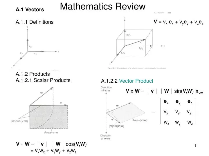
e x e y e z v x v y v z w x w y w z. =. A.1 Vectors A.1.1 Definitions. V = v x e x + v y e y + v z e z. Mathematics Review. A.1.2 Products A.1.2.1 Scalar Products. A.1.2.2 Vector Product. V x W = | v || W | sin( V,W ) n vw. V . W = | v | | W | cos( V,W )

E N D
exeyez vx vy vz wx wy wz = A.1 Vectors A.1.1 Definitions V = vxex + vyey + vzez Mathematics Review A.1.2 Products A.1.2.1 Scalar Products A.1.2.2 Vector Product V x W = |v||W|sin(V,W) nvw V.W = |v| |W|cos(V,W) = vxwx + vywy + vzwz
A.2 Tensors A.2.1 Definitions A tensor (2nd order) has nine components, for example, a stress tensor can be expressed in rectangular coordinates listed in the following: A.2.2 Product The tensor product of two vectors v and w, denoted as vw, is a tensor defined by [A.2-1] [A.2-2] Explanation (Borisenko, p64)
The vector product of a tensor t and a vector v, denoted by t.v is a vector defined by [A.2-3] The product between a tensor vv and a vector n is a vector [A.2-5]
Physical quantity Multiplication sign Scalar Vector Tensor None X ‧ : Order 0 1 2 0 -1 -2 -4 The scalar product of two tensors s and t, denoted as s:t, is a scalar defined by [A.2-6] The scalar product of two tensors vw and t is [A.2-7] Table A.1-1 Orders of physical quantities and their multiplication signs
A.3 Differential Operators A.3.1 Definitions The vector differential operation , called “del”, has components similar to those of a vector. However, unlike a vector, it cannot stand alone and must operate on a scalar, vector, or tensor function. In rectangular coordinates it is defined by [A.3-1] The gradient of a scalar field s, denoted as▽s, is a vector defined by [A.3-2] A.3.2 Products The divergence of a vector field v, denoted as ▽‧v is a scalar . [A.3-5] Flux is defined as the amount that flows through a unit area per unit time Flow rate is the volume of fluid which passes through a given surface per unit time
Similarly [A.3-5] For the operation of [A.3-7] For the operation of ▽‧▽s, we have [A.3-8] In other words [A.3-9] Where the differential operator▽2, called Laplace operator, is defined as [A.3-10] For example: Streamline is defined as a line everywhere tangent to the velocity vector at a given instant and can be described as a scale function of f. Lines of constant f are streamlines of the flow for inviscid irrotational flow in the xy plane ▽2f=0
When the flow is irrotational, The curl of a vector field v, denoted by ▽x v, is a vector like the vector product of two vectors. [A.3-11] Like the tensor product of two vectors, ▽v is a tensor as shown: [A.3-12]
Like the vector product of a vector and a tensor, ▽‧t is a vector. [A.3-13] From Eq. [A.2-2] [A.3-14] [A.3-15] It can be shown that
A.4 Divergence Theorem A.4.1 Vectors Let Ω be a closed region in space surrounded by a surface A and n the outward- directed unit vector normal to the surface. For a vector v [A.4-1] This equation , called the gauss divergence theorem, is useful for converting from a surface integral to a volume integral. A.4.2 Scalars For a scale s [A.4-2] A.4.3 Tensors For a tensor t or vv [A.4-3] [A.4-4]
A.5 Curvilinear Coordinates For many problems in transport phenomena, the curvilinear coordinates such as cylindrical and spherical coordinates are more natural than rectangular coordinates. A point P in space, as shown in Fig. A.5.1, can be represented by P(x,y,z) in rectangular coordinates, P(r, θ,z) in cylindrical coordinates, or P(r, θ,ψ) in spherical coordinates. A.5.1 Cartesian Coordinates ey y For Cartesian coordinates, as shown in A.5-1(a), the differential increments of a control unit in x, y and z axis are dx, dy , and dz, respectively. dy ex P(x,y,z) dz dx ez x z Fig. A.5-1(a)
A.5.1 Cylindrical Coordinates For cylindrical coordinates, as shown in A.5-1(b), the variables r, θ, and z are related to x, y, and z. x = r cosθ [A.5-1] y = r sinθ [A.5-2] z = z [A.5-3] The differential increments of a control unit, as shown in Fig. A.5-1(b)*, in r, q, and z axis are dr, rdq , and dz, respectively. A vector v and a tensor τcan be expressed as follows: v = er vr + eθvθ + ezvz and Fig. A.5-1(b) Fig. A.5-1(b)*
A.5.2 Spherical Coordinates For spherical coordinates, as shown in A.5-1(c), the variables r, θ, and ψ are related to x, y, and z as follows x= r sinq cosf [A.5-6] y = r sinq sinf [A.5-7] z = r cosq [A.5-8] Fig. A.5-1(c) The differential increments of a control unit, as shown in Fig. A.5-1(c)*, in r, θ, and φ axis are dr, rdθ , and rsinθdφ , respectively. A vector v and a tensor τ can be expressed as follows: [A.5-9] φ θ θ θ θ θ [A.5-10] φ φ Fig. A.5-1(c)*
A.5.3 Differential Operators Vectors, tensors, and their products in curvilinear coordinates are similar in form to those in curvilinear coordinates. For example, if v = er in cylindrical coordinates, the operation of τ.er can be expressed in [A.5-11], and it can be expressed in [A.5-12] when in spherical coordinates [A.5-11] [A.5-12] In curvilinear coordinates, ▽ assumes different forms depending on the orders of the physical quantities and the multiplication sign involved. For example, in cylindrical coordinates [A.5-13] Whereas in spherical coordinates, [A.5-14]
The equations for ▽s, ▽‧v, ▽ xv, and ▽2s in rectangular, cylindrical, and spherical coordinates are given in Tables A.5-1, A.5-2, and A.5-3, respectively. φ θ θ θ θ θ φ φ