Download

1 / 45
450 likes | 511 Views
All-Pairs Shortest Paths. Csc8530 – Dr. Prasad Jon A Preston March 17, 2004. Outline. Review of graph theory Problem definition Sequential algorithms Properties of interest Parallel algorithm Analysis Recent research References. Graph Terminology. G = (V, E) W = weight matrix

E N D
All-Pairs Shortest Paths Csc8530 – Dr. Prasad Jon A Preston March 17, 2004
Outline • Review of graph theory • Problem definition • Sequential algorithms • Properties of interest • Parallel algorithm • Analysis • Recent research • References
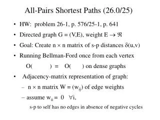
Graph Terminology • G = (V, E) • W = weight matrix • wij = weight/length of edge (vi, vj) • wij = ∞ if vi and vj are not connected by an edge • wii = 0 • Assume W has positive, 0, and negative values • For this problem, we cannot have a negative-sum cycle in G
0 1 2 3 4 Weighted Graph and Weight Matrix v1 v0 5 -4 v2 3 1 2 7 9 6 v3 v4
Directed Weighted Graph and Weight Matrix v3 v0 -2 1 7 v1 v2 -1 2 5 9 6 3 4 0 1 2 3 4 5 v4 v5
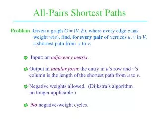
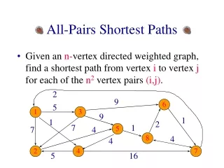
All-Pairs Shortest Paths Problem Defined • For every pair of vertices vi and vj in V, it is required to find the length of the shortest path from vi to vj along edges in E. • Specifically, a matrix D is to be constructed such that dij is the length of the shortest path from vi to vj in G, for all i and j. • Length of a path (or cycle) is the sum of the lengths (weights) of the edges forming it.
Sample Shortest Path v3 v0 -2 1 7 v1 v2 2 -1 5 9 6 3 4 v4 v5 Shortest path from v0 to v4 is along edges (v0, v1), (v1, v2), (v2, v4) and has length 6
Disallowing Negative-length Cycles • APSP does not allow for input to contain negative-length cycles • This is necessary because: • If such a cycle were to exist within a path from vi to vj, then one could traverse this cycle indefinitely, producing paths of ever shorter lengths from vi to vj. • If a negative-length cycle exists, then all paths which contain this cycle would have a length of -∞.
Recent Work on Sequential Algorithms • Floyd-Warshall algorithm is Θ(V3) • Appropriate for dense graphs: |E| = O(|V|2) • Johnson’s algorithm • Appropriate for sparse graphs: |E| = O(|V|) • O(V2 log V + V E) if using a Fibonacci heap • O(V E log V) if using binary min-heap • Shoshan and Zwick (1999) • Integer edge weights in {1, 2, …, W} • O(W Vωp(V W)) where ω ≤ 2.376 and p is a polylog function • Pettie (2002) • Allows real-weighted edges • O(V2 log log V + V E) Strassen’s Algorithm (matrix multiplication)
Properties of Interest • Let denote the length of the shortest path from vi to vj that goes through at most k - 1 intermediate vertices (k hops) • = wij (edge length from vi to vj) • If i ≠ j and there is no edge from vi to vj, then • Also, • Given that there are no negative weighted cycles in G, there is no advantage in visiting any vertex more than once in the shortest path from vi to vj. • Since there are only n vertices in G,
Guaranteeing Shortest Paths • If the shortest path from vi to vj contains vr and vs (where vr precedes vs) • The path from vr to vs must be minimal (or it wouldn’t exist in the shortest path) • Thus, to obtain the shortest path from vi to vj, we can compute all combinations of optimal sub-paths (whose concatenation is a path from vi to vj), and then select the shortest one vi vr vs vj MIN MIN MIN ∑ MINs
Iteratively Building Shortest Paths v1 w1j v2 w2j … vn vi vj wnj
Recurrence Definition • For k > 1, • Guarantees O(log k) steps to calculate vi vl vj MIN MIN ≤ k/2 vertices ≤ k/2 vertices ≤ k vertices
Computing D • Let Dk = matrix with entries dij for 0 ≤ i, j ≤ n - 1. • Given D1, compute D2, D4, … , Dm • D = Dm • To calculate Dk from Dk/2, use special form of matrix multiplication • ‘’ → ‘’ • ‘’ → ‘min’
“Modified” Matrix Multiplication Step 2: forr = 0 toN – 1 dopar Cr = Ar + Br end Step 3: form = 2qto 3q – 1 do forallr N (rm = 0) dopar Cr = min(Cr, Cr(m))
“Modified” Example P101 P100 2 3 2 -4 P000 P001 From 9.2, after step (1.3) 1 -1 1 -2 3 -1 3 -2 P110 P010 P011 P111 4 -3 4 -4
“Modified” Example (step 2) P101 P100 5 -2 P000 P001 From 9.2, after modified step 2 0 -1 2 1 P110 P010 P011 P111 1 0
“Modified” Example (step 3) P101 P100 P000 P001 MIN MIN From 9.2, after modified step 3 0 -2 1 0 MIN MIN P110 P010 P011 P111
Hypercube Setup • Begin with a hypercube of n3 processors • Each has registers A, B, and C • Arrange them in an nnn array (cube) • Set A(0, j, k) = wjk for 0 ≤ j, k ≤ n – 1 • i.e processors in positions (0, j, k) contain D1 = W • When done, C(0, j, k) contains APSP = Dm
0 1 2 3 4 5 Setup Example D1 = Wjk = A(0, j, k) = v3 v0 -2 1 7 v1 v2 -1 2 5 9 6 3 4 v4 v5
APSP Parallel Algorithm Algorithm HYPERCUBE SHORTEST PATH (A,C) Step 1: forj = 0 ton - 1 dopar fork = 0 ton - 1 dopar B(0, j, k) = A(0, j, k) end for end for Step 2: fori = 1 todo (2.1) HYPERCUBE MATRIX MULTIPLICATION(A,B,C) (2.2) forj = 0 ton - 1 dopar for k = 0 ton - 1 dopar (i) A(0, j, k) = C(0, j, k) (ii) B(0, j, k) = C(0, j, k) end for end for end for
An Example 0 1 2 3 4 5 0 1 2 3 4 5 D1 = D2 = 0 1 2 3 4 5 0 1 2 3 4 5 D4 = D8 =
Analysis • Steps 1 and (2.2) require constant time • There are iterations of Step (2.1) • Each requires O(log n) time • The overall running time is t(n) = O(log2n) • p(n) = n3 • Cost is c(n) = p(n) t(n) = O(n3 log2n) • Efficiency is
Recent Research • Jenq and Sahni (1987) compared various parallel algorithms for solving APSP empirically • Kumar and Singh (1991) used the isoefficiency metric (developed by Kumar and Rao) to analyze the scalability of parallel APSP algorithms • Hardware vs. scalability • Memory vs. scalability
Isoefficiency • For “scalable” algorithms (efficiency increases monotonically as p remains constant and problem size increases), efficiency can be maintained for increasing processors provided that the problem size also increases • Relates the problem size to the number of processors necessary for an increase in speedup in proportion to the number of processors used
Isoefficiency (cont) • Given an architecture, defines the“degree of scalability” • Tells us the required growth in problem size to be able to efficiently utilize an increasing number of processors • Ex:Given an isoefficiency of kp3If p0 and w0, speedup = 0.8p0 (efficiency = 0.8)If p1 = 2p0, to maintain efficiency of 0.8w1 = 23w0 = 8w0 • Indicates the superiority of one algorithm over another only when problem sizes are increased in the range between the two isoefficiency functions
Isoefficiency (cont) • Given an architecture, defines the“degree of scalability” • Tells us the required growth in problem size to be able to efficiently utilize an increasing number of processors • Ex:Given an isoefficiency of kp3If p0 and w0, speedup = 0.8p0 (efficiency = 0.8)If w1 = 2w0, to maintain efficiency of 0.8p1 = 23w0 = 8w0 • Indicates the superiority of one algorithm over another only when problem sizes are increased in the range between the two isoefficiency functions Given an isoefficiency of kp3If p0 and w0, speedup = 0.8p0 (efficiency = 0.8)If p1 = 2p0, to maintain efficiency of 0.8w1 = 23w0 = 8w0
Memory Overhead Factor (MOF) • Ratio: Total memory required for all processors Memory required for the same problems size on single processor • We’d like this to be lower!
Architectures Discussed • Shared Memory (CREW) • Hypercube (Cube) • Mesh • Mesh with Cut-Through Routing • Mesh with Cut-Through and Multicast Routing • Also examined fast and slow communication technologies
Parallel APSP Algorithms • Floyd Checkerboard • Floyd Pipelined Checkerboard • Floyd Striped • Dijkstra Source-Partition • Dijkstra Source-Parallel
General Parallel Algorithm (Floyd) Repeat steps 1 through 4 for k := 1 to n Step 1: If this processor has a segment of Pk-1[*,k], then transmit it to all processors that need it Step 2: If this processor has a segment of Pk-1[k,*], then transmit it to all processors that need it Step 3: Wait until the needed segments of Pk-1[*,k] and Pk-1[k,*] have been received Step 4: For all i, j in this processor’s partition, computePk[i,j] := min {Pk-1[i,j], Pk-1[i,k] + Pk-1[k,j]}
Floyd Checkerboard Each “cell” is assigned to adifferent processor, and thisprocessor is responsible forupdating the cost matrixvalues at each iteration ofthe Floyd algorithm. Steps 1 and 2 of the GPFinvolve each of the processors sending theirdata to the “neighbor”columns and rows.
Floyd Pipelined Checkerboard Similar to the preceding. Steps 1 and 2 of the GPFinvolve each of the processors sending theirdata to the “neighbor”columns and rows. The difference is that theprocessors are notsynchronized and computeand send data ASAP (orsends as soon as it receives).
Floyd Striped Each “column” is assigned adifferent processor, and thisprocessor is responsible forupdating the cost matrixvalues at each iteration ofthe Floyd algorithm. Step 1 of the GPFinvolves each of the processors sending theirdata to the “neighbor”columns. Step 2 is notneeded (since the columnis contained within theprocessor).
Dijkstra Source-Partition • Assumes Dijkstra’s Single-source Shortest Path is equally distributed over p processors and executed in parallel • Processor p finds shortest paths from each vertex in it’s set to all other vertices in the graph • Fortunately, this approach involves no inter-processor communication • Unfortunately, only n processors can be kept busy • Also, memory overhead is high since each processors has a copy of the weight matrix
Dijkstra’s Source-Parallel • Motivated by keeping more processors busy • Run n copies of the Dijkstra’s SSP • Each copy runs on processors (p > n)
Calculating Isoefficiency • Example: Floyd Checkerboard • At most n2 processors can be kept busy • n must grow as Θ(√p) due to problem structure • By Floyd (sequential), Te = Θ(n3) • Thus isoefficiency is √(p3) = Θ(p1.5) • But what about communication…
Calculating Isoefficiency (cont) • ts = message startup time • tw = per-word communication time • tc = time to compute next iteration value for one cell in matrix • m = number words sent • d = number hops between nodes • Hypercube: • (ts + tw m) log d = time to deliver m words • 2 (ts + tw m) log p = barrier synchronization time (up & down “tree”) • d = √p • Step 1 = (ts + tw n/√p) log √p • Step 2 = (ts + tw n/√p) log √p • Step 3 (barrier synch) = 2(ts + tw) log p • Step 4 = tcn2/p Isoefficiency = Θ(p1.5(log p)3)
Mathematical Details How are n and p related?
Calculating Isoefficiency (cont) • ts = message startup time • tw = per-word communication time • tc = time to compute next iteration value for one cell in matrix • m = number words sent • d = number hops between nodes • Mesh: • Step 1 = • Step 2 = • Step 3 (barrier synch) = • Step 4 = Te Isoefficiency = Θ(p3+p2.25) = Θ(p3)
Isoefficiency and MOF forAlgorithm & Architecture Combinations
Comparing Metrics • We’ve used “cost” previously this semester(cost = pTp) • But notice that the cost of all of the architecture-algorithm combinations discussed here is Θ(n3) • Clearly some are more scalable than others • Thus isoefficiency is a useful metric when analyzing algorithms and architectures
References • Akl S. G. Parallel Computation: Models and Methods. Prentice Hall, Upper Saddle River NJ, pp. 381-384,1997. • Cormen T. H., Leiserson C. E., Rivest R. L., and Stein C. Introduction to Algorithms (2nd Edition). The MIT Press, Cambridge MA, pp. 620-642, 2001. • Jenq J. and Sahni S. All Pairs Shortest Path on a Hypercube Multiprocessor. In International Conference on Parallel Processing. pp. 713-716, 1987. • Kumar V. and Singh V. Scalability of Parallel Algorithms for the All Pairs Shortest Path Problem. Journal of Parallel and Distributed Computing, vol. 13, no. 2, Academic Press, San Diego CA, pp. 124-138, 1991. • Pettie S. A Faster All-pairs Shortest Path Algorithm for Real-weighted Sparse Graphs. In Proc. 29th Int'l Colloq. on Automata, Languages, and Programming (ICALP'02), LNCS vol. 2380, pp. 85-97, 2002.