Download
1 / 46
460 likes | 609 Views
Tutorial for solution of Assignment week 39 “A. Time series without seasonal variation Use the data in the file 'dollar.txt'. “. “Construct a time series graph of the fluctuations of the dollar exchange rate, y t , for the period 1994-1998.”.

E N D
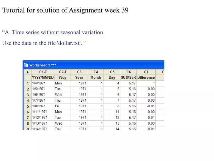
Tutorial for solution of Assignment week 39 “A. Time series without seasonal variation Use the data in the file 'dollar.txt'. “
“Construct a time series graph of the fluctuations of the dollar exchange rate, yt, for the period 1994-1998.”
Note! The time scale is best set to index here as the days are not consecutive in time series (Saturdays, Sundays and other holidays are not present)
“Construct also a point plot for all pairs (yt-1 , yt) and try to visually estimate how strong the correlation between two consecutive observations is (=autocorrelation).”
Strong positive autocorrelation! “How do the estimated autocorrelations change with increasing timelags between observations?” To estimate the autocorrelation function, copy the relevant rows (data for 1994-1998) of column $US/SEK to a new column and use the autocorrelation function estimation on that column
As was deduced from the scatter plot, the autocorrelations are strongly positive. The autocorrelations do not change very much with increasing time lags. Note that this is what we see when the time series is non-stationary (has a trend).
“Construct a time series graph of the changes zt = yt - yt-1 of the dollar exchange rate. Then try to judge upon how the estimated autocorrelations for the series zt change with the time lag between observations and check your judgement by estimating the autocorrelations.” The changes are already present in the column Difference. The analogous procedures are applied to this column to produce the time series graph and the estimated acf plot, i.e. by including only values where column Year is 1994.
Noisy plot As previously plot zt vs. zt – 1 Seems to be no autocorrelation at all
“B. Time series with seasonal variation Use the time series of monthly discharge in the lake Hjälmaren (‘Hjalmarenmonth.txt’), which you have used in the assignment for week 36. Compute the autocorrelation function (Minitab: StatTime seriesAutocorrelation…) for the variable Discharge.m.”
“Deseasonalise the time series and make a new graph of the seasonally adjusted values. Try to visually estimate how the autocorrelations look like and check your judgement by computing the autocorrelation function.” Additive model for deseasonalization seems best!
Indicates positive autocorrelation Plot DESE1(t) vs. DESE1(t-1)
“C. Forecasting with autoregressive models Data set: The Dollar Exchange rates Consider again the time series of dollar exchange rates for the period 1994-1998. Then use the Minitab time series module ARIMA (see further below) to estimate the parameters in an AR(1)-model (1 nonseasonal autoregressive parameter) and plot the observed values together with forecasts for a period of 20 days after the last observed time-point.” Use the already created column of $US/SEK exchange rates from 1994-1998 (there is no opportunity in Minitab’s ARIMA module to just analyze a subset of a column like in the graphing modules)
Forecasts for a 20 days period are requested. (Origin field is left blank analogously to previous modules) See next slide! Three new columns should be entered here!
Must be checked (not default) Should always by checked for diagnostic purposes
Final Estimates of Parameters Type Coef SE Coef T P AR 1 0.9971 0.0026 385.44 0.000 Constant 0.021782 0.001280 17.02 0.000 Mean 7.4405 0.4371 Number of observations: 1229 Residuals: SS = 2.45718 (backforecasts excluded) MS = 0.00200 DF = 1227 Modified Box-Pierce (Ljung-Box) Chi-Square statistic Lag 12 24 36 48 Chi-Square 9.0 22.9 33.3 38.2 DF 10 22 34 46 P-Value 0.529 0.410 0.504 0.786 Significant! Keep in mind for comparison with next model OK!
Forecasts from period 1229 95 Percent Limits Period Forecast Lower Upper Actual 1230 7.79895 7.71122 7.88668 1231 7.79790 7.67401 7.92178 1232 7.79685 7.64535 7.94836 1233 7.79581 7.62112 7.97050 1234 7.79477 7.59974 7.98979 1235 7.79373 7.58040 8.00706 1236 7.79270 7.56261 8.02278 1237 7.79167 7.54605 8.03728 1238 7.79064 7.53051 8.05077 1239 7.78961 7.51581 8.06342 1240 7.78859 7.50184 8.07534 1241 7.78757 7.48850 8.08664 1242 7.78655 7.47572 8.09739 1243 7.78554 7.46344 8.10764 1244 7.78453 7.45161 8.11745 1245 7.78352 7.44018 8.12687 1246 7.78252 7.42912 8.13592 1247 7.78152 7.41839 8.14464 1248 7.78052 7.40798 8.15306 1249 7.77952 7.39786 8.16119 These forecasts and prediction limits are stored in columns C12, C13 and C14 (as entered in dialog box)
Seems to be OK (as was confirmed by the Ljung-Box statistic)
Use the stored prediction limits to calculate the widths of the prediction intervals The column widths_1 (C15) will later be compared with the widths from another model
“Investigate also if the forecasts can improve by instead using an AR(2)-model.” Don’t forget to enter new columns here!
Final Estimates of Parameters Type Coef SE Coef T P AR 1 1.0107 0.0286 35.35 0.000 AR 2 -0.0138 0.0285 -0.48 0.629 Constant 0.023161 0.001280 18.09 0.000 Mean 7.4372 0.4110 Number of observations: 1229 Residuals: SS = 2.45873 (backforecasts excluded) MS = 0.00201 DF = 1226 Modified Box-Pierce (Ljung-Box) Chi-Square statistic Lag 12 24 36 48 Chi-Square 10.2 24.0 34.3 39.3 DF 9 21 33 45 P-Value 0.337 0.292 0.403 0.710 Non-significant! Slightly larger than in AR(1)-model Still OK!
Make a time series plot of the intervals widths from the two analyses.
Slightly wider prediction intervals with AR(2)-model (widths_2) Forecasts do not improve with AR(2)-model
“Finally perform a residual analysis of the errors in the one-step-ahead forecasts (can be asked for under the “Graph” button in the dialog box. By residuals we mean here the errors in the one-step-ahead forecasts). Are there any signs of serial correlations in the residuals?” AR(1): AR(2): No signs of serial correlations in resiaduals in any of the models
“D. ARIMA models and differentiation In this task you will first have to judge upon whether you need to differentiate the current time series ( zt= yt - yt-1 ) before forecasting with an ARMA-model can be applied. Then you shall try different models with a number of parameters to find the model that gives the least one-step-ahead prediction errors on the average. Finally you shall make some residual plots to investigate if the selected model of forecasting can be improved.” “Forecasting monthly dollar exchange rates in Danish crowns (DKK) Data set: The Dollar-Danish Crowns Exchange rates”
“D.1. The need for differentiation Construct a time series graph for the monthly means of dollar exchange rates in Danish crowns (file ‘DKK.txt’). Then estimate the autocorrelations and display them in a graph. Does the time series show any obvious upward or downward trend?”
Note that the y-axisdo not start at zero! A slight upward trend may be concluded “Are there any signs of long-time oscillations in the time series (that can be seen from the time series graph)?” Yes, there seem to be a cyclical variation with cycle periods longer than a year.
“Is there a fast cancel-out in the autocorrelations?” No, the cancel-out is not fast (although the spikes come quickly within the red limits) “Is there need for differentiation to get a time series suitable for ARMA-modelling?” Probably, but not certainly!
“D.2 Fitting different ARMA-models Calculate the estimated autocorrelations possibly after differentiation of the original series and display these estimates in a graph.” Without differentiation: (Slowly) decreasing postive autocorrelations. One positive spike (at lag 1) in SPAC Either this is a non-stationary time series or an AR(1)-time series with a close to 1.
With first-order differentiation (use the ready series of differences): No obvious pattern in any of these two plots. The differentiated series may be an ARMA-series
“Then try to predict the dollar exchange rate by combining differentiation with ARMA-models of different orders.” Strategy: On original series, try AR(1) On differentiated series, try AR(1), AR(2), MA(1), MA(2), ARMA(1,1), ARMA(1,2), ARMA(2,1) and ARMA(2,2) Compare the values of MS from each model. This measure corresponds with one-step-ahead prediction errors on the average.
None of the models on the differentiated series produces better MS value than the AR(1) on original series, but MS seems to decrease with larger complexity.
“What happens if one tries to fit a very complex model with a lot of parameters to the observations?” Study e.g. ARMA(3,3) and ARMA(4,4) on the differentiated series:
Final Estimates of Parameters Type Coef SE Coef T P AR 1 -0.1113 0.3369 -0.33 0.742 AR 2 0.4786 0.2274 2.10 0.038 AR 3 0.3689 0.3237 1.14 0.258 MA 1 -0.1098 0.2941 -0.37 0.710 MA 2 0.4351 0.2136 2.04 0.045 MA 3 0.6165 0.2846 2.17 0.033 Constant 0.000924 0.001931 0.48 0.634 Differencing: 1 regular difference Number of observations: Original series 95, after differencing 94 Residuals: SS = 3.25649 (backforecasts excluded) MS = 0.03743 DF = 87 Modified Box-Pierce (Ljung-Box) Chi-Square statistic Lag 12 24 36 48 Chi-Square 4.9 17.3 26.4 39.5 DF 5 17 29 41 P-Value 0.425 0.431 0.606 0.537 ARMA(3,3) Even lower than in ARMA(2,2) No severe problems but not all parameters are significant!
No severe problems here either, but spikes seem to increase with lag!
Unable to reduce sum of squares any further Final Estimates of Parameters Type Coef SE Coef T P AR 1 0.4196 2.3514 0.18 0.859 AR 2 0.4329 0.4304 1.01 0.317 AR 3 0.0536 1.2079 0.04 0.965 AR 4 -0.0652 0.7425 -0.09 0.930 MA 1 0.4119 2.3452 0.18 0.861 MA 2 0.3871 0.4030 0.96 0.340 MA 3 0.3397 1.0707 0.32 0.752 MA 4 -0.1736 1.2715 -0.14 0.892 Constant 0.000597 0.001779 0.34 0.738 Differencing: 1 regular difference Number of observations: Original series 95, after differencing 94 Residuals: SS = 3.26434 (backforecasts excluded) MS = 0.03840 DF = 85 Estimation problems! ARMA(4,4) None of the parameters are significant! Estimation problems and an increase in MS. Increased!
The conclusion must be that an AR(1)-model on original data seems to be the best. “D.3. Residual analysis Construct a graph for the residuals (the one-step-ahead prediction errors) and examine visually if anything points to a possible improvement of the model.” SAC and SPAC of residuals do not indicate that another ARIMA-model should be used.
There do not seem to be any violations of the assumption of normal distribution and constant variance either.