Download
1 / 30
310 likes | 531 Views
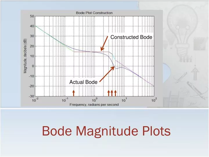
Bode Magnitude Plots. Constructed Bode. Professor Walter W. Olson Department of Mechanical, Industrial and Manufacturing Engineering University of Toledo. Actual Bode. Outline of Today’s Lecture. Review Poles and Zeros Plotting Functions with Complex Numbers Root Locus

E N D
Bode Magnitude Plots Constructed Bode Professor Walter W. Olson Department of Mechanical, Industrial and Manufacturing Engineering University of Toledo Actual Bode
Outline of Today’s Lecture • Review • Poles and Zeros • Plotting Functions with Complex Numbers • Root Locus • Plotting the Transfer Function • Effects of Pole Placement • Root Locus Factor Responses • Frequency Response • Reading the Bode Plot • Computing Logarithms of |G(s)| • Bode Magnitude Plot Construction
Root Locus • The root locus plot for a system is based on solving the system characteristic equation • The transfer function of a linear, time invariant, system can be factored as a fraction of two polynomials • When the system is placed in a negative feedback loop the transfer function of the closed loop system is of the form • The characteristic equation is • The root locus is a plot of this solution for positive real values of K • Because the solutions are the system modes, this is a powerful design tool
Root Locus • The root locus plot for a system is based on solving the system characteristic equation • The transfer function of a linear, time invariant, system can be factored as a fraction of two polynomials • When the system is placed in a negative feedback loop the transfer function of the closed loop system is of the form • The characteristic equation is • The root locus is a plot of this solution for positive real values of K • Because the solutions are the system modes, this is a powerful design tool
The effect of placement on the root locus jw Imaginary axis jwd sin-1(z) wn Real Axis s s = -zwn • The magnitude of the vector to • pole location is the natural frequency • of the response, wn • The vertical component (the imaginary • part) is the damped frequency, wd • The angle away from the vertical is the • inverse sine of the damping ratio, z
The effect of placement on the root locus jw Imaginary axis jwd sin-1(z) wn Real Axis s s = -zwn • The magnitude of the vector to • pole location is the natural frequency • of the response, wn • The vertical component (the imaginary • part) is the damped frequency, wd • The angle away from the vertical is the • inverse sine of the damping ratio, z
Frequency Response General form of linear time invariant (LTI) system was previously expressed as We now want to examine the case where the input is sinusoidal. The response of the system is termed its frequency response.
Frequency Response • The response to the input is amplified by M and time shifted by the phase angle. • To represent this response we need two curves: • one for the magnitude at any frequency and • one for phase shift • These curves when plotted are called the Bode Plot of the system
Reading the Bode Plot Amplifies Attenuates Input Response The magnitude is in decibels decade also, cycle Note: The scale for w is logarithmic
What is a decibel? • The decibel (dB) is a logarithmic unit that indicates the ratio of a physical quantity relative to a specified or implied reference level. A ratio in decibels is ten times the logarithm to base 10 of the ratio of two power quantities. (IEEE Standard 100 Dictionary of IEEE Standards Terms, Seventh Edition, The Institute of Electrical and Electronics Engineering, New York, 2000; ISBN 0-7381-2601-2; page 288) Because decibels is traditionally used measure of power, the decibel value of a magnitude, M, is expressed as 20 Log10(M) • 20 Log10(1)=0 … implies there is neither amplification or attenuation • 20 Log10(100)= 40 decibels … implies that the signal has been amplified 100 times from its original value • 20 Log10(0.01)= -40 decibels … implies that the signal has been attenuated to 1/100 of its original value
Note • The book does not plot the Magnitude of the Bode Plot in decibels. • Therefore, you will get different results than the book where decibels are required. • Matlab uses decibels.
Sketching Semilog Paper • First, determine how many cycles you will need: • Ideally, you will need at least one cycle below the smallest zero or pole and • At least one cycle above the largest pole or zero • Example • Knowing how many cycles needed, divide the sketch area into these regions
Sketching Semilog Paper • For this example assume 100 0.1 1.0 10 Frequency w rps
Sketching Semilog Paper • For each cycle, • Estimate the 1/3 point and label this 2 x the starting point for the cycle • Estimate the midway point and label this 3 * the starting point for the cycle • At the 2/3 point, label this 5 x * the starting point for the cycle • Half way between 3 and 5 place a tic representing 4 • Halfway between 5 and 10 place a tic and label this 7 • Halfway between 5 and 7, place a tic for 6 • Divide the space between 7 and 10 into thirds and label these 8 and 9 • These are not exact but useful for sketching purposes 0.2 0.3 0.5 0.7 2 3 5 7 20 30 50 70 100 0.1 1.0 10 Frequency w rps
Computing Logarithms of |G(s)| Therefore, in plotting the magnitude portion of the Bode plot, we can compute each term separately and then add them up for the result
Computing Logarithms of G(s) Since this does not vary with the frequency it a constant that will be added to all of the other factors when combined and has the effect of moving the complete plot up or down When this is plotted on a semilog graph (w the abscissa) this is a straight line with a slope of 20p (p is negative if the sp term is in the denominator of G(s)) … without out any other terms it would pass through the point (w,MdB) = (1,0) p is often called the “type” of the system
Static Error Constants • If the system is of type 0 at low frequencies will be level. • A type 0 system, (that is, a system without a pole at the origin,)will have a static position error, Kp, equal to • If the system is of type 1 (a single pole at the origin) it will have a slope of -20 dB/dec at low frequencies • A type 1 system will have a static velocity error, Kv, equal to the value of the -20 dB/dec line where it crosses 1 radian per second • If the system is of type 2 ( a double pole at the origin) it willhave a slope of -40 dB/dec at low frequencies • A type 2 system has a static acceleration error,Ka, equal to the value of the -40 dB/dec line where it crosses 1 radian per second
Computing Logarithms of G(s) a is called the break frequency for this factor For frequencies of less than arad/sec, this is plotted as a horizontal line at the level of 20Log10 a, For frequencies greater than arad/sec, this is plotted as a line with a slope of ± 20 dB/decade, the sign determined by position in G(s)
Example • Assume we have the transfer function • To compute the magnitude part of the Bode plot +
Example Constructed Plot Actual Bode Magnitude Plot • Bode plot of Our plotting technique produces an “asymptotic Bode Plot”
Computing Logarithms of G(s) wn is called the break frequency for this factor For frequencies of less than wnrad/sec, this is plotted as a horizontal line at the level of 40Log10wn, For frequencies greater than wnrad/sec, this is plotted as a line with a slope of ± 40 dB/decade, the sign determined by position in G(s)
Example • Construct a Bode magnitude plot of + Note: there are two lines here!
Example Actual Bode Magnitude Asymptotic Bode Magnitude
Corrections • You seen on the asymptotic Bode magnitude plots, there were deviations at the break frequencies. Note that these could be either positive of negative corrections depending on whether or not the term is in the numerator or denominator For (s+a) type terms For quadratic terms pertains to a phase correction which will be discussed next class
Bode Plot Construction • When constructing Bode plots, there is no need to draw the curves for each factor: this was done to show you where the parts came from. • The best way to construct a Bode plot is to first make a table of the critical frequencies and record that action to be taken at that frequency. • You want to start at least one decade below the smallest break frequency and end at least one decade above the last break frequency. This will determine how semilog cycles you will need for the graph paper. • This will be shown by the following example.
Example • Plot the Bode magnitude plot of
Example Constructed Bode Actual Bode
Note: This form has certain advantages: 1) the time constants of the 1st order terms can be directly read 2) When constructing Bode plots the part of the curves up to the break frequencies are 0 (20Log101=0). The level parts have been taken up in the constant gain, Kt
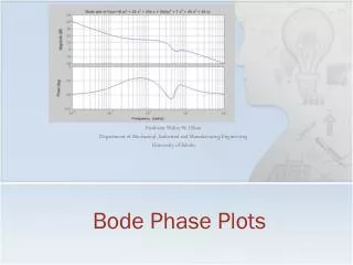
Summary • Frequency Response • Reading the Bode Plot • Computing Logarithms of |G(s)| • Bode Magnitude Plot Construction Next: Bode Phase Plots