Download
1 / 103
1.04k likes | 1.05k Views
Trees. Dr. B. Prabhakaran {praba@utdallas.edu}. Application Examples. Useful for locating items in a list Used in Huffman coding algorithm Study games like checkers and chess to determine winning strategies Weighted trees used to model various categories of problems. Trees.

E N D
Trees Dr. B. Prabhakaran {praba@utdallas.edu}
Application Examples • Useful for locating items in a list • Used in Huffman coding algorithm • Study games like checkers and chess to determine winning strategies • Weighted trees used to model various categories of problems
Trees Definition: A connected undirected graph with no simple circuits Characteristics - No multiple edges - No loops
Example UT Dallas School of Engineering School of Management School of Social Sciences School of Arts CS EE TE Cohort MBA
Which of the following graphs are trees? e e a a b a b b c c a d f c f f d e d b f d c e A B C D A & B : Trees C: Not a Tree (Cycle abdcfa) D: Not a Tree (Not connected). However it is a forest i.e. unconnected graphs
Tree Theorem Theorem 1 : An undirected Graph is a tree if and only if there is a unique simple path between any two of its vertices Proof (=>) The graph is a Tree and it does not have cycles. If there were cycles then there will be more than one simple path between two vertices. Hence, there is a unique simple path between every pair of vertices Proof (<=) There exists a unique simple path between any pair of vertices. Therefore the graph is connected and there are no cycles in the graph. Hence, the graph is a tree
Tree terminology Rooted tree:one vertex designated as root and every edge directed away Parent: u is the parent of v iff (if and only if) there is an edge directed from u to v Child:v is called the child of u Every non-root node has a unique parent (?)
Tree terminology Siblings:vertices with same parent Ancestors:all vertices on path from the root to this vertex, excluding the vertex Descendants:Descendants of vertex v are all vertices that have v as an ancestor Internal Nodes: Nodes that have children External or Leaf Nodes: Nodes that have no children
Given : Tree rooted at A Find: Descendants (B), Ancestor (A), Siblings (G) ? A Root Node = A Internal Nodes = B, C, E and F B C E D F K G I J H External Nodes = D,G, H ,I, J and K
Definition - Level • The level of vertex v in a rooted tree is the length of the unique path from the root to v
What is the level of Ted? Lou Hal Max Ken Sue Ed Joe Ted
Definition - Height • The height of a rooted tree is the maximum of the levels of its vertices
What is the height? Lou Hal Max Ken Sue Ed Joe Ted
Definition: m-ary trees • Rooted tree where every vertex has no more than ‘m’ children • Full m-ary if every internal vertex has exactly ‘m’ children (i.e., except leaf/external vertices). • m=2 gives a binary tree
Definition: Binary Tree • Every internal vertex has a maximum of 2 children • An ordered rooted tree is a rooted tree where the children of each internal vertex are ordered. • In an ordered binary tree, the two possible children of a vertex are called the left child and the right child, if they exist.
An Ordered Binary Tree Lou Hal Max Ken Sue Ed Joe Ted
Definition: Balanced • A rooted binary tree of height h is called balanced if all its leaves are at levels h or h-1
Is this tree balanced? Lou Hal Max Ken Sue Ed Joe Ted
Tree Property 1 Theorem 2 : A tree with n vertices has n-1 edges Proof: By induction Basis Step: for n = 1 there are (1 – 1) 0 edges Inductive Step: We assume that n vertices has n – 1 edges . We need to prove that n + 1 vertices have n edges. A tree with n + 1 vertices can be achieved by adding an edge from a vertex of the tree to the new vertex (why 1 edge ?). The total number of edges is (n – 1 + 1 = n).
Tree Property 2 Theorem 3: A full m-ary tree with i internal vertices contains n = mi +1 vertices Proof: i internal vertices have m children. Therefore, we have mi vertices. Since the root is not a child we have n = mi + 1 vertices.
Tree Property 3 Theorem 4: A full m-ary tree with 1) n vertices has i = (n-1)/m internal vertices and l = [(m-1)n+1]/m leaves 2) i internal vertices has n = mi + 1 vertices and l = (m-1)i+1 leaves 3) l leaves has n = (ml-1)/(m-1) vertices and i = (l-1)/(m-1) internal vertices
Tree Property 4 Theorem 5 – Proof for 1) l: Number of leaves i: Number of internal vertices n: total number of vertices. By theorem 3, n = mi + 1, and we have n = l + i (why ?) n = mi + 1 => i = (n-1)/m By subsitution in n = l + i • l = n – i • l = n – (n-1)/m • [(m-1)n+1]/m
Tree Property 4 Theorem 5 – Proof for 2) l: Number of leaves i: Number of internal vertices n: total number of vertices. By theorem 3, n = mi + 1, and we have n = l + i By subsitution in n = l + i • l + i = mi + 1 • l = (m-1) i + 1
Tree Property 4 Theorem 5 – Proof for 3) l: Number of leaves i: Number of internal vertices n: total number of vertices. By theorem 3, n = mi + 1, and we have n = l + i (i = n – l) By subsitution of i in n = mi + 1 • n = m (n –l) + 1 • n (m -1) = (ml -1) • n = (ml -1)/ (m -1) By subsitution of n in i = n – l we have i = (l – 1)/(m – 1)
Tree Property 5 Theorem 6: There are at most mh leaves in a m-ary tree of height h Proof: By Induction Basic Step: m-ary tree of height 1 => leaves = m which is true since the root has m-ary children
Tree Property 5 Inductive Step: • Assume that the result is true for tree of height less than h • Let Tree T be m-ary of height h • To build T we can add m such sub-tree of height ≤ h -1 such that the root node acts as the child to the root of T • T has ≤ m.mh -1 ≤ mh
Applications of trees • Binary Search Trees • Decision Trees • Prefix Codes • Game Trees
Binary Search Trees (BST) Applications • A Binary Search Tree can be used to store items in its vertices • It enables efficient searches
Definition: BST A special kind of binary tree in which: • Each vertex contains a distinct key value, • The key values in the tree can be compared using “greater than” and “less than”, and • The key value of each vertex in the tree is less than every key value in its right subtree, and greater than every key value in its left subtree.
Shape of a binary search tree Depends on its key values and their order of insertion. Example: Insert the elements 6, 3, 4, 2, 10 in that order . The first value to be inserted is put into the root 6
Shape of a binary search tree Inserting 3 into the BST 6 3
Shape of a binary search tree Inserting 4 into the BST 6 3 4
Shape of a binary search tree Inserting 4 into the BST 6 3 4 2
Shape of a binary search tree Inserting 10 into the BST 6 10 3 4 12 2
Binary search tree algorithm • procedureinsertion (T:binary search tree, X: item) • v:= root of T • {a vertex not present in T has the value null} • while v != null and label(v) != x • begin • if x < label(v) then • if left child of v != nullthen v:=left child of v • else add new vertex as left child of v and set v:= null • else • if right child of v != nullthen v:=right child of v • else add new vertex as right child of v to T and set v := null • end • if root of T = nullthen add a vertex v to the tree and label it with x • elseif v is null or label(v) != x then label new vertex with x and let v be this new vertex • {v = location of x}
Codes Text Encoding • Our next goal is to develop a code that represents a given text as compactly as possible. • A standard encoding is ASCII, which represents every character using 7 bits: • “An English sentence” = 133 bits ≈ 17 bytes • 1000001 (A) 1101110 (n) 0100000 ( ) 1000101 (E) 1101110 (n) 1100111 (g)1101100 (l) 1101001 (i) 1110011 (s) 1101000 (h) • 0100000 ( ) 1110011 (s) 1100101 (e) 1101110 (n) 1110100 (t) 1100101 (e) 1101110 (n) 1100011 (c)1100101 (e)
Codes Text Encoding Of course, this is wasteful because we can encode 12 characters in 4 bits: ‹space› = 0000 A = 0001 E = 0010 c = 0011 e = 0100 g = 0101 h = 0110i = 0111 l = 1000 n = 1001 s = 1010 t = 1011 Then we encode the phrase as 0001 (A) 1001 (n) 0000 ( ) 0010 (E) 1001 (n) 0101 (g) 1000 (l) 0111 (i)1010 (s) 0110 (h) 0000 ( ) 1010 (s) 0100 (e) 1001 (n) 1011 (t) 0100 (e)1001 (n) 0011 (c) 0100 (e) This requires 76 bits ≈ 10 bytes
Codes Text Encoding An even better code is given by the following encoding: ‹space› = 000 A = 0010 E = 0011 s = 010 c = 0110 g = 0111 h = 1000 i = 1001 l = 1010 t = 1011 e = 110 n = 111 Then we encode the phrase as 0010 (A) 111 (n) 000 ( ) 0011 (E) 111 (n) 0111 (g) 1010 (l) 1001 (i) 010 (s) 1000 (h) 000 ( ) 010 (s) 110 (e) 111 (n) 1011 (t) 110 (e) 111 (n) 0110 (c) 110 (e) This requires 65 bits ≈ 9 bytes
Codes Codes That Can Be Decoded Fixed-length codes: • Every character is encoded using the same number of bits. • To determine the boundaries between characters, we form groups of w bits, where w is the length of a character. • Examples: • ASCII • Our first improved code Prefix codes: • No character is the prefix of another character. • Examples: • Fixed-length codes • Huffman codes
Why Prefix Codes ? • Consider a code that is not a prefix code:a = 01 m = 10 n = 111 o = 0 r = 11 s = 1 t = 0011 • Now you send a fan-letter to your favorite movie star. One of the sentences is “You are a star.”You encode “star” as “1 0011 01 11”. • Your idol receives the letter and decodes the text using your coding table:100110111 = 10 0 11 0 111 = “moron”
0 1 0 1 0 1 0 1 0 1 0 1 0 1 s n e ‹spc› 1 0 1 0 1 0 1 0 g c t A E h i l Representing a Prefix-Code Dictionary Our example:‹space› = 000 A = 0010 E = 0011 s = 010 c = 0110 g = 0111 h = 1000 i = 1001 l = 1010 t = 1011 e = 110 n = 111
f:5 e:9 c:12 b:13 d:16 a:45 Huffman’s Algorithm Huffman(C) 1n← |C| 2Q←C 3fori = 1..n – 1 4do allocate a new node z 5 left[z] ←x← Delete-Min(Q) 6 right[z] ←y← Delete-Min(Q) 7f [z] ←f [x] + f [y] 8 Insert(Q, z) 9return Delete-Min(Q)
14 f:5 e:9 c:12 b:13 d:16 a:45 Huffman’s Algorithm Huffman(C) 1n← |C| 2Q←C 3fori = 1..n – 1 4do allocate a new node z 5 left[z] ←x← Delete-Min(Q) 6 right[z] ←y← Delete-Min(Q) 7f [z] ←f [x] + f [y] 8 Insert(Q, z) 9return Delete-Min(Q)
14 c:12 a:45 b:13 d:16 f:5 e:9 Huffman’s Algorithm Huffman(C) 1n← |C| 2Q←C 3fori = 1..n – 1 4do allocate a new node z 5 left[z] ←x← Delete-Min(Q) 6 right[z] ←y← Delete-Min(Q) 7f [z] ←f [x] + f [y] 8 Insert(Q, z) 9return Delete-Min(Q)
25 14 c:12 a:45 b:13 d:16 f:5 e:9 Huffman’s Algorithm Huffman(C) 1n← |C| 2Q←C 3fori = 1..n – 1 4do allocate a new node z 5 left[z] ←x← Delete-Min(Q) 6 right[z] ←y← Delete-Min(Q) 7f [z] ←f [x] + f [y] 8 Insert(Q, z) 9return Delete-Min(Q)
14 25 d:16 a:45 f:5 c:12 b:13 e:9 Huffman’s Algorithm Huffman(C) 1n← |C| 2Q←C 3fori = 1..n – 1 4do allocate a new node z 5 left[z] ←x← Delete-Min(Q) 6 right[z] ←y← Delete-Min(Q) 7f [z] ←f [x] + f [y] 8 Insert(Q, z) 9return Delete-Min(Q)
30 14 25 d:16 a:45 f:5 c:12 b:13 e:9 Huffman’s Algorithm Huffman(C) 1n← |C| 2Q←C 3fori = 1..n – 1 4do allocate a new node z 5 left[z] ←x← Delete-Min(Q) 6 right[z] ←y← Delete-Min(Q) 7f [z] ←f [x] + f [y] 8 Insert(Q, z) 9return Delete-Min(Q)
25 30 a:45 14 b:13 d:16 c:12 f:5 e:9 Huffman’s Algorithm Huffman(C) 1n← |C| 2Q←C 3fori = 1..n – 1 4do allocate a new node z 5 left[z] ←x← Delete-Min(Q) 6 right[z] ←y← Delete-Min(Q) 7f [z] ←f [x] + f [y] 8 Insert(Q, z) 9return Delete-Min(Q)