Download
1 / 19
260 likes | 573 Views
Segmentation by Morphological Watersheds. Introduction. Based on visualizing an image in 3D. imshow(I,[ ]). mesh(I). Introduction. Instead of working on an image itself, this technique is often applied on its gradient image .

E N D
Introduction • Based on visualizing an image in 3D imshow(I,[ ]) mesh(I)
Introduction • Instead of working on an image itself, this technique is often applied on its gradient image. • In this case, each object is distinguished from the background by its up-lifted edges
Basic Definitions • I: 2D gray level image • DI: Domain of I • Path P of length l between p and q in I • A (l+1)-tuple of pixels (p0=p,p1,…,pl=q) such that pi,pi+1are adjacent (4 adjacent, 8 adjacent, or m adjacent, see Section 2.5) • l(P): The length of a given path P • Minimum • A minimum M of I is a connected plateau of pixels from which it is impossible to reach a point of lower altitude without having to climb
Basic Definitions • Instead of working on an image itself, this technique is often applied on its gradient image. • Three types of points • Points belonging to a regional minimum • Catchment basin / watershed of a regional minimum • Points at which a drop of water will certainly fall to a single minimum • Divide lines / Watershed lines • Points at which a drop of water will be equally likely to fall to more than one minimum • Crest lines on the topographic surface • This technique is to identify all the third type of points for segmentation
Basic Steps • Piercing holes in each regional minimum of I • The 3D topography is flooded from below gradually • When the rising water in distinct catchment basins is about to merge, a dam is built to prevent the merging
3. The dam boundaries correspond to the watershed lines to be extracted by a watershed segmentation algorithm - Eventually only constructed dams can be seen from above
Dam Construction • Based on binary morphological dilation • At each step of the algorithm, the binary image in obtained in the following manner • Initially, the set of pixels with minimum gray level are 1, others 0. • In each subsequent step, we flood the 3D topography from below and the pixels covered by the rising water are 1s and others 0s. (See previous slides)
Notations • M1, M2: • Sets of coordinates of points in the two regional minima • Cn-1(M1), Cn-1(M2) • Sets of coordinates of points in the catchment basins associated with M1 M2 at stage n-1 of flooding (catchment basins up to the flooding level) • C[n-1] • Union of Cn-1(M1), Cn-1(M2)
Dam Construction • At flooding step n-1, there are two connected components. At flooding step n, there is only one connected component • This indicates that the water between the two catchment basins has merged at flooding step n • Use “q” to denote the single connected component • Steps • Repeatedly dilate Cn-1(M1), Cn-1(M2) by the 3×3 structuring element shown, subject to the following condition • Constrained to q (center of the structuring element can not go beyond q during dilation
Dam Construction • The dam is constructed by the points on which the dilation would cause the sets being dilated to merge. • Resulting one-pixel thick connected path • Setting the gray level at each point in the resultant path to a value greater than the maximum gray value of the image. Usually max+1
n-1 Mi C(Mi) T(n) Watershed Transform • Denote M1, M2, …, MR as the sets of the coordinates of the points in the regional minima of an (gradient) image g(x,y) • Denote C(Mi) as the coordinates of the points in the catchment basin associated with regional minimum Mi. • Denote the minimum and maximum gray levels of g(x,y) as min and max • Denote T[n] as the set of coordinates (s,t) for which g(s,t) < n • Flood the topography in integer flood increments from n=min+1 to n=max+1 • At each flooding, the topography is viewed as a binary image
Watershed Transform • Denote Cn(Mi) as the set of coordinates of points in the catchment basin associated with minimum Mi at flooding stage n. • Cn(Mi)= C(Mi) T[n] • Cn(Mi)=T[n] • Denote C[n] as the union of the flooded catchment basin portions at stage n: • Initialization • Let C[min+1]=T[min+1] • At each step n, assume C[n-1] has been constructed. The goal is to obtain C[n] from C[n-1] n-1 Mi C(Mi) T(n) Cn(Mi) C(n)
Dam n-1 n-2 Mi C(Mi) T(n-1) C(n-1) T(n) q2 q3 q1 C(n) Watershed Transform • Denote Q[n] as the set of connected components in T[n]. • For each qQ[n], there are three possibilities • q C[n-1] is empty (q1) • A new minimum is encountered • q is incorporated into C[n-1] to form C[n] • q C[n-1] contains one connected component of C[n-1] (q2) • q is incorporated into C[n-1] to form C[n] • q C[n-1] contains more than one connected components of C[n-1] (q3) • A ridge separating two or more catchment basins has been encountered • A dam has to be built within q to prevent overflow between the catchment basins • Repeat the procedure until n=max+1 Cn-1(Mi)
A B C D Examples 1 Watershed Transform of Binary Image A: Original image B: Negative of image A C: Distance transform of B D: Watershed transform of C Distance transform of a binary image is defined by the distance from every pixel to the nearest non-zero valued pixel
a b c d Examples 2 a: Original image b: Gradient image of image a c: Watershed lines obtained from image b (oversegmentation) Each connected region contains one local minimum in the corresponding gradient image d: Watershed lines obtained from smoothed image b
The Use of Markers • Internal markers are used to limit the number of regions by specifying the objects of interest • Like seeds in region growing method • Can be assigned manually or automatically • Regions without markers are allowed to be merged (no dam is to be built) • External markers those pixels we are confident to belong to the background • Watershed lines are typical external markers and they belong the same (background) region
Watershed Based Image Segmentation • Use internal markers to obtain watershed lines of the gradient of the image to be segmented. • Use the obtained watershed lines as external markers • Each region defined by the external markers contains a single internal marker and part of the background • The problem is reduced to partitioning each region into two parts: object (containing internal markers) and a single background (containing external markers) • Global thresholding, region growing, region splitting and merging, or watershed transform
A B C D E F G MATLAB Example • A: Original image f • B: Direct watershed transform result using the following commands • L=watershed(g) • wr = L ==0 • g is the gradient image of A • C: shows all of the regional minima of g using “rm=imregionalmin(g)” • D: internal markers obtained by • im = imextendedmin(g,2) • fim = f; • fim(im) = 175; • E: External markers using • Lim = watershed(bwdist(im)) • em = Lim ==0 • F: Modified gradient image obtained from internal and external markers • g2 = imimposemin(g, im | em) • G: Final segmentation result • L2 = watershed(g2) • f2 = f; • f2(L2 == 0) = 255