Download
1 / 31
320 likes | 474 Views
1. Nominal Measures of Association 2. Ordinal Measure s of Association. ASSOCIATION. Association The strength of relationship between 2 variables Knowing how much variables are related may enable you to predict the value of 1 variable when you know the value of another

E N D
1. Nominal Measures of Association2. Ordinal Measure s of Association
ASSOCIATION • Association • The strength of relationship between 2 variables • Knowing how much variables are related may enable you to predict the value of 1 variable when you know the value of another • As with test statistics, the proper measure of association depends on how variables are measured
Significance vs. Association • Association = strength of relationship • Test statistics = how different findings are from null • They do capture the strength of a relationship • t = number of standard errors that separate means • Chi-Square = how different our findings are from what is expected under null • If null is no relationship, then higher Chi-square values indicate stronger relationships. • HOWEVER --- test statistics are also influenced by other stuff (e.g., sample size)
MEASURES OF ASSOCIATION FOR NOMINAL-LEVEL VARIABLES “Chi-Square Based” Measures • 2 indicates how different our findings are from what is expected under null • 2 also gets larger with higher sample size (more confidence in larger samples) • To get a “pure” measure of strength, you have to remove influence of N • Phi • Cramer's V
PHI • Phi (Φ) = 2 √ N • Formula standardizes 2 value by sample size • Measure ranges from 0 (no relationship) to values considerably >1 • (Exception: for a 2x2 bivariate table, upper limit of Φ= 1)
PHI • Example: • 2 x 2 table • 2=5.28 • LIMITATION OF Φ: • Lack of clear upper limit makes Φan undesirable measure of association
CRAMER’S V • Cramer’s V = 2 √ (N)(Minimum of r-1, c-1) • Unlike Φ, Cramer’s V will always have an upper limit of 1, regardless of # of cells in table • For 2x2 table, Φ & Cramer’s V will have the same value • Cramer’s V ranges from 0 (no relationship) to +1 (perfect relationship)
2-BASED MEASURES OF ASSOCIATION • Sample problem 1: • The chi square for a 5 x 3 bivariate table examining the relationship between area of Duluth one lives in & type of movie preference is 8.42, significant at .05 (N=100). Calculate & interpret Cramer’s V. • ANSWER: • (Minimum of r-1, c-1) = 3-1 = 2 • Cramer’s V = .21 • Interpretation: There is a relatively weak association between area of the city lived in and movie preference.
2-BASED MEASURES OF ASSOCIATION • Sample problem 2: • The chi square for a 4 x 4 bivariate table examining the relationship between type of vehicle driven & political affiliation is 12.32, sig. at .05 (N=300). Calculate & interpret Cramer’s V. • ANSWER: • (Minimum of r-1, c-1) = 4 -1 = 3 • Cramer’s V = .12 • Interpretation: There is a very weak association between type of vehicle driven & political affiliation.
SUMMARY: 2 -BASED MEASURES OF ASSOCIATION • Limitation of Φ& Cramer’s V: • No direct or meaningful interpretation for values between 0-1 • Both measure relative strength (e.g., .80 is stronger association than .40), but have no substantive meaning; hard to interpret • “Rules of Thumb” for what is a weak, moderate, or strong relationship vary across disciplines
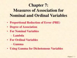
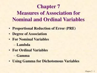
LAMBDA (λ) • PRE (Proportional Reduction in Error) is the logic that underlies the definition & computation of lambda • Tells us the reduction in error we gain by using the IV to predict the DV • Range 0-1 (i.e., “proportional” reduction) • E1 – Attempt to predict the category into which each case will fall on DV or “Y” while ignoring IV or “X” • E2– Predict the category of each case on Y while taking X into account • The stronger the association between the variables the greater the reduction in errors
LAMBDA: EXAMPLE 1 • Does risk classification in prison affect the likelihood of being rearrested after release? (2=43.7)
LAMBDA: EXAMPLE • Find E1 (# of errors made when ignoring X) • E1 = N – (largest row total) = 205 -120 = 85
LAMBDA: EXAMPLE • Find E2 (# of errors made when accounting for X) • E2 = (each column’s total – largest N in column) = (75-50) + (40-20) + (90-75) = 25+20+15 = 60
CALCULATING LAMBDA: EXAMPLE • Calculate Lambda λ = E1 – E2 =85-60=25= 0.294 E1 85 85 • Interpretation – when multiplied by 100, λ indicates the % reduction in error achieved by using X to predict Y, rather than predicting Y “blind” (without X) • 0.294 x 100 = 29.4% - “Knowledge of risk classification in prison improves our ability to predict rearrest by 29%.”
LAMBDA: EXAMPLE 2 • What is the strength of the relationship between citizens’ race and attitude toward police? • (obtained chi square is > 5.991 (2[critical]) • Calculate & interpret lambda to answer this question
LAMBDA: EXAMPLE 2 E1 = N – (largest row total) 455 – 230 = 225 E2 = (each column’s total – largest N in column) (120 – 80) + (245 – 150) + (90 – 55) = 40 + 95 + 35 = 170 λ = E1 – E2 =225 - 170= 55 = 0.244 E1 225 225 INTERPRETATION: • 0. 244 x 100 = 24.4% - “Knowledge of an individual’s race improves our ability to predict attitude towards police by 24%”
SPSS EXAMPLE • IS THERE A SIGNIFICANT RELATIONSHIP B/T GENDER & VOTING BEHAVIOR? • If so, what is the strength of association between these variables? • ANSWER TO Q1: “YES”
SPSS EXAMPLE • ANSWER TO QUESTION 2: • By either measure, the association between these variables appears to be weak
2 LIMITATIONS OF LAMBDA 1. Asymmetric • Value of the statistic will vary depending on which variable is taken as independent 2. Misleading when one of the row totals is much larger than the other(s) • For this reason, when row totals are extremely uneven, use a chi square-based measure instead
ORDINAL MEASURE OF ASSOCIATION • GAMMA • For examining STRENGTH & DIRECTION of “collapsed” ordinal variables (<6 categories) • Like Lambda, a PRE-based measure • Range is -1.0 to +1.0
GAMMA • Logic: Applying PRE to PAIRS of individuals
GAMMA • CONSIDER KENNY-DEB PAIR • In the language of Gamma, this is a “same” pair • direction of difference on 1 variable is the same as direction on the other • If you focused on the Kenny-Eric pair, you would come to the same conclusion
GAMMA • NOW LOOK AT THE TIM-JOEY PAIR • In the language of Gamma, this is a “different” pair • direction of difference on one variable is opposite of the difference on the other
GAMMA • Logic: Applying PRE to PAIRS of individuals • Formula: same – different same + different
GAMMA • If you were to account for all the pairs in this table, you would find that there were 9 “same” & 9 “different” pairs • Applying the Gamma formula, we would get: 9 – 9 = 0 = 0.0 18 18
GAMMA • 3-case example • Applying the Gamma formula, we would get: 3 – 0 = 3 = 1.00 3 3
Gamma: Example 1 • Examining the relationship between: • FEHELP (“Wife should help husband’s career first”) & • FEFAM (“Better for man to work, women to tend home”) • Both variables are ordinal, coded 1 (strongly agree) to 4 (strongly disagree)
Gamma: Example 1 • Based on the info in this table, does there seem to be a relationship between these factors? • Does there seem to be a positive or negative relationship between them? • Does this appear to be a strong or weak relationship?
GAMMA • Do we reject the null hypothesis of independence between these 2 variables? • Yes, the Pearson chi square p value (.000) is < alpha (.05) • It’s worthwhile to look at gamma. • Interpretation: • There is a strong positive relationship between these factors. • Knowing someone’s view on a wife’s “first priority” improves our ability to predict whether they agree that women should tend home by 75.5%.
USING GSS DATA • Construct a contingency table using two ordinal level variables • Are the two variables significantly related? • How strong is the relationship? • What direction is the relationship?