Download
1 / 35
350 likes | 368 Views
Dive into the world of parallel algorithms and complexities through 5 essential computations on 4 architectures. Understand semigroup computation, parallel prefix, packet routing, broadcasting, and sorting.

E N D
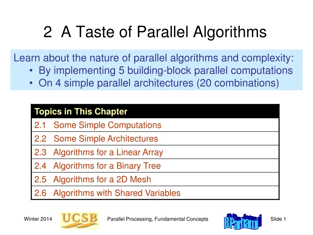
2 A Taste of Parallel Algorithms Learn about the nature of parallel algorithms and complexity: • By implementing 5 building-block parallel computations • On 4 simple parallel architectures (20 combinations) Parallel Processing, Fundamental Concepts
2.1.SOME SIMPLE COMPUTATIONS Five fundamental building-block computations are: 1. Semigroup (reduction, fan-in) computation 2. Parallel prefix computation 3. Packet routing 4. Broadcasting, and its more general version, multicasting 5. Sorting records in ascending/descending order of their keys Parallel Processing, Fundamental Concepts
2.1.SOME SIMPLE COMPUTATIONS • Semigroup Computation: • Let ⊗ be an associative binary operator; For example: • (x ⊗ y ) ⊗ z = x ⊗ (y ⊗ z ) for all x, y, z ∈ S. A semigroup is simply a pair (S, ⊗), where S is a set of elements on which ⊗ is defined. • Semigroup (also known as reduction or fan-in ) computation is defined as: Given a list of n values x0, x1, . . . , xn–1, compute x0 ⊗ x1 ⊗ . . . ⊗ xn–1 . Parallel Processing, Fundamental Concepts
2.1.SOME SIMPLE COMPUTATIONS • Semigroup Computation: • Common examples for the operator ⊗ include +, ×, ∧ , ∨ , ⊕, ∩, ∪, max, min. • The operator ⊗ may or may not be commutative, i.e., it may or may not satisfy x ⊗ y = y ⊗ x (all of the above examples are, but the carry computation, e.g., is not). • while the parallel algorithm can compute chunks of the expression using any partitioning scheme, the chunks must eventually be combined in left-to-right order. Parallel Processing, Fundamental Concepts
2.1.SOME SIMPLE COMPUTATIONS • Parallel Prefix Computation: • With the same assumptions as in the Semigroup Computation, a parallel prefix computation is defined as simultaneously evaluating all of the prefixes of the expression x0 ⊗ x 1 . . . ⊗ xn–1; • Output: x0, x0 ⊗ x1, x0 ⊗ x1 ⊗ x2, . . . , x 0 ⊗ x1 ⊗ . . .⊗ xn–1. • Note that the ith prefix expression is si= x0 ⊗ x1 ⊗ . . . ⊗ xi. The comment about commutativity, or lack thereof, of the binary operator ⊗ applies here as well. Parallel Processing, Fundamental Concepts
2.1.SOME SIMPLE COMPUTATIONS Fig.2.1. Semigroup computation on a uniprocessor Parallel Processing, Fundamental Concepts
2.1.SOME SIMPLE COMPUTATIONS • Packet Routing: • A packet of information resides at Processor iand must be sent to Processor j. • The problem is to route the packet through intermediate processors, if needed, such that it gets to the destination as quickly as possible Parallel Processing, Fundamental Concepts
2.1.SOME SIMPLE COMPUTATIONS • Broadcasting • Given a value a known at a certain processor i, disseminate it to all p processors as quickly as possible, so that at the end, every processor has access to, or “knows,” the value. This is sometimes referred to as one-to-all communication. • The more general case of this operation, i.e., one-to-many communication, is known as multicasting. Parallel Processing, Fundamental Concepts
2.1.SOME SIMPLE COMPUTATIONS Sorting: Rather than sorting a set of records, each with a key and data elements, we focus on sorting a set of keys for simplicity. Our sorting problem is thus defined as: Given a list of n keys x0, x1, . . . , xn–1, and a total order ≤ on key values, rearrange the n keys as Xinondescending order. Parallel Processing, Fundamental Concepts
2.2.SOME SIMPLE ARCHITECTURES We define four simple Parallel Architectures: 1. Linear array of processors 2. Binary tree of processors 3. Two-dimensional mesh of processors 4. Multiple processors with shared variables Parallel Processing, Fundamental Concepts
2.2.SOME SIMPLE ARCHITECTURES 1. Linear array of processors: Fig. 2.2 A linear array of nine processors and its ring variant. Max node degree d = 2 Network diameter D = p – 1 ( p/2 ) Bisection width B = 1 ( 2 ) Parallel Processing, Fundamental Concepts
2.2.SOME SIMPLE ARCHITECTURES 2. Binary Tree Max node degree d = 3 Network diameter D = 2 log2p (- 1 ) Bisection width B = 1 Parallel Processing, Fundamental Concepts
Max node degree d = 4 Network diameter D = 2p – 2 ( p ) Bisection width Bp ( 2p ) 2.2.SOME SIMPLE ARCHITECTURES 3. 2D Mesh Fig. 2.4 2D mesh of 9 processors and its torus variant. Parallel Processing, Fundamental Concepts
2.2.SOME SIMPLE ARCHITECTURES 4. Shared Memory Max node degree d = p – 1 Network diameter D = 1 Bisection width B = p/2p/2 Costly to implement Not scalable But . . . Conceptually simple Easy to program Fig. 2.5 A shared-variable architecture modeled as a complete graph. Parallel Processing, Fundamental Concepts
2.3.ALGORITHMS FOR A LINEAR ARRAY 1.Semigroup Computation: Fig. 2.6 Maximum-finding on a linear array of nine processors. For general semigroup computation: Phase 1: Partial result is propagated from left to right Phase 2: Result obtained by processor p – 1 is broadcast leftward Parallel Processing, Fundamental Concepts
2.3.ALGORITHMS FOR A LINEAR ARRAY 2.Parallel Prefix Computation: Fig. 2.8 Computing prefix sums on a linear array with two items per processor. Parallel Processing, Fundamental Concepts
2.3.ALGORITHMS FOR A LINEAR ARRAY • 3.Packet Routing: • To send a packet of information from Processor ito Processor j on a linear array, we simply attach a routing tag with the value j – ito it. • The sign of a routing tag determines the direction in which it should move (+ = right, – = left) while its magnitude indicates the action to be performed (0 = remove the packet, nonzero = forward the packet). With each forwarding, the magnitude of the routing tag is decremented by 1 Parallel Processing, Fundamental Concepts
2.3.ALGORITHMS FOR A LINEAR ARRAY • 4.Broadcasting: • If Processor iwants to broadcast a value a to all processors, it sends an rbcast(a) (read r-broadcast) message to its right neighbor and an lbcast(a) message to its left neighbor. • Any processor receiving an rbcast(a ) message, simply copies the value a and forwards the message to its right neighbor (if any). Similarly, receiving an lbcast(a) message causes a to be copied locally and the message forwarded to the left neighbor. • The worst-case number of communication steps for broadcasting is p – 1. Parallel Processing, Fundamental Concepts
2.3.ALGORITHMS FOR A LINEAR ARRAY 5.Sorting: Fig. 2.9 Sorting on a linear array with the keys input sequentially from the left. Parallel Processing, Fundamental Concepts
2.3.ALGORITHMS FOR A LINEAR ARRAY Fig. 2.10 Odd-even transposition sort on a linear array. T(1) = W(1) = p log2pT(p) = pW(p) p2/2 S(p) = log2pR(p) = p/(2 log2p) Parallel Processing, Fundamental Concepts
2.4.ALGORITHMS FOR A Binary Tree 1. Semigroup Computation Reduction computation and broadcasting on a binary tree. Parallel Processing, Fundamental Concepts
2.4.ALGORITHMS FOR A BINARY TREE 2. Parallel Prefix Computation Fig. 2.11 Scan computation on a binary tree of processors. Parallel Processing, Fundamental Concepts
2.4.ALGORITHMS FOR A BINARY TREE • Some applications of the parallel prefix computation Ranks of 1s in a list of 0s/1s: Data: 0 0 1 0 1 0 0 1 1 1 0 Prefix sums: 0 0 1 1 2 2 2 3 4 5 5 Ranks of 1s: 1 2 3 4 5 Priority arbitration circuit: Data: 0 0 1 0 1 0 0 1 1 1 0 Dim’d prefix ORs: 0 0 0 1 1 1 1 1 1 1 1 Complement: 1 1 1 0 0 0 0 0 0 0 0 AND with data: 0 0 1 0 0 0 0 0 0 0 0 Parallel Processing, Fundamental Concepts
2.4.ALGORITHMS FOR A BINARY TREE 3. Packet Routing If dest = self Then remove the packet Else if dest< self or dest>maxr then rout upward Else if dest<= maxl then rout leftward else rout rightward end if end if End if Preorder indexing Parallel Processing, Fundamental Concepts
2.4.ALGORITHMS FOR A BINARY TREE 4.Sorting if you have 2 items then do nothing else if you have 1 item that came from the left (right) then get the smaller item from the right (left) child else get the smaller item from each child endif endif Parallel Processing, Fundamental Concepts
2.4.ALGORITHMS FOR A BINARY TREE Fig. 2.12 The first few steps of the sorting algorithm on a binary tree. Parallel Processing, Fundamental Concepts
2.5.ALGORITHMS FOR A 2D MESH • Semigroup computation: • To perform a semigroup computation on a 2D mesh, do the semigroup computation in each row and then in each column. • For example, in finding the maximum of a set of p values, stored one per processor, the row maximums are computed first and made available to every processor in the row. Then column maximums are identified. • This takes 4 p – 4 steps on a p-processor square mesh Parallel Processing, Fundamental Concepts
2.5.ALGORITHMS FOR A 2D MESH • 2. Parallel Prefix computation: • This can be done in three phases, assuming that the processors (and their stored values) are indexed in row-major order: • do a parallel prefix computation on each row • do a diminished parallel prefix computation in the rightmost column. • broadcast the results in the rightmost column to all of the elements in the respective rows and combine with the initially computed row prefix value. Parallel Processing, Fundamental Concepts
2.5.ALGORITHMS FOR A 2D MESH 3. Packet Routing: To route a data packet from the processor in Row r, Column c, to the processor in Row r', Column c', we first route it within Row r to Column c'. Then, we route it in Column c' from Row r to Row r' 4. Broadcasting: Broadcasting is done in two phases: (1) broadcast the packet to every processor in the source node’s row and (2) broadcast in all columns Parallel Processing, Fundamental Concepts
2.5.ALGORITHMS FOR A 2D MESH 5. Sorting: Figure 2.14. The Shearsort algorithm on 3*3 mesh Parallel Processing, Fundamental Concepts
2.5.ALGORITHMS FOR A 2D MESH 5. Sorting: Figure 2.14. The Shearsort algorithm on 3*3 mesh Parallel Processing, Fundamental Concepts
2.6.ALGORITHMS WITH SHARED VARIABLES • Semigroup Computation: • Each processor obtains the data items from all other processors and performs the semigroup computation independently. Obviously, all processors will end up with the same result • 2. Parallel Prefix Computation: • Similar to the semigroup computation, except that each processor only obtains data items from processors with smaller indices. • 3. Packet Routing • Trivial in view of the direct communication path between any pair • of processors. Parallel Processing, Fundamental Concepts
2.6.ALGORITHMS WITH SHARED VARIABLES 4. Broadcasting: Trivial, as each processor can send a data item to all processors directly. In fact, because of this direct access, broadcasting is not needed; each processor already has access to any data item when needed. 5. Sorting: The algorithm to be described for sorting with shared variables consists of two phases: ranking and data permutation. Ranking consists of determining the relative order of each key in the final sorted list. Parallel Processing, Fundamental Concepts
2.6.ALGORITHMS WITH SHARED VARIABLES • If each processor holds one key, then once the ranks are determined, the jth-ranked key can be sent to Processor j in the data permutation phase, requiring a single parallel communication step. Processor i is responsible for ranking its own key xi. • This is done by comparing xi to all other keys and counting the number of keys that are smaller than xi. In the case of equal key values, processor indices are used to establish the relative order. Parallel Processing, Fundamental Concepts
THE END Parallel Processing, Fundamental Concepts