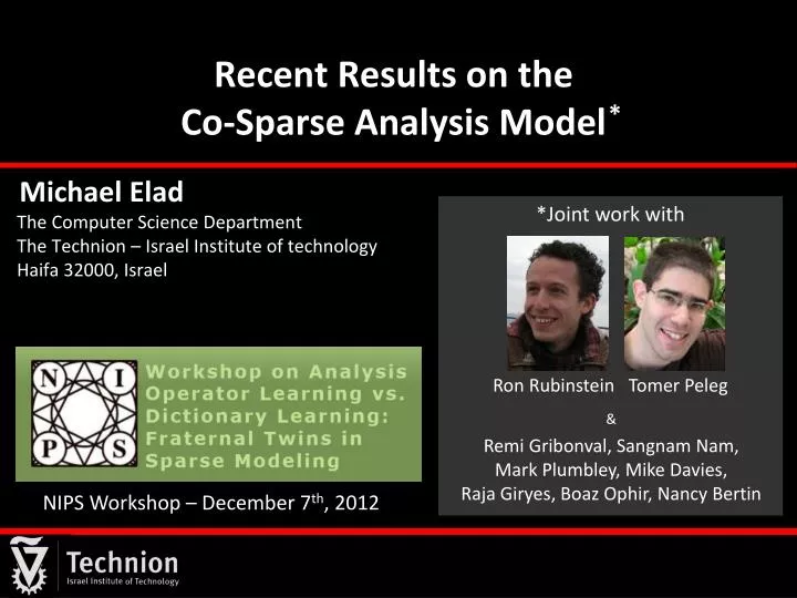
Recent Results on the Co-Sparse Analysis Model

1. * Recent Results on theCo-Sparse Analysis Model *Joint work with Ron Rubinstein TomerPeleg Michael Elad The Computer Science Department The Technion – Israel Institute of technology Haifa 32000, Israel & Remi Gribonval, SangnamNam, Mark Plumbley, Mike Davies, Raja Giryes, Boaz Ophir, Nancy Bertin NIPS Workshop – December 7th, 2012

2. Stock Market Heart Signal CT & MRI Radar Imaging Still Image Voice Signal Traffic info Informative Data  Inner Structure • It does not matter what is the data you are working on – if it carries information, it must have an inner structure. • This structure = rules the data complies with. • Signal/image processing relies on exploiting these “rules” by adopting models. • A model = mathematical construction describing the properties of the signal. • In the past decade, sparsity-based models has been drawing major attention.

3. Sparsity-Based Models Sparsity and Redundancy can be Practiced in (at least) two different ways Analysis Synthesis The attention to sparsity-based models has been given mostly to the synthesis option, leaving the analysis almost untouched. For a long-while these two options were confused, even considered to be (near)-equivalent. Well … now we know better !! The two are VERY DIFFERENT The co-sparse analysis model is a very appealing alternative to the synthesis model, it has a great potential for signal modeling. This Talk’s Message:

4. Agenda Part I - Background Recalling the Synthesis Sparse Model Part II - Analysis Turning to the Analysis Model Part III – THR Performance Revealing Important Dictionary Properties Part IV – Dictionaries Analysis Dictionary-Learning and Some Results Part V – We Are Done Summary and Conclusions

5. Part I - Background Recalling the Synthesis Sparse Model

6. The Sparsity-Based Synthesis Model D • We assume the existence of a synthesis dictionary DIR dn whose columns are the atom signals. • Signals are modeled as sparselinear combinations of the dictionary atoms: • We seek a sparsityof , meaning that it is assumed to contain mostly zeros. • We typically assume that n>d: redundancy. • This model is typically referred to as thesynthesissparse and redundant representation model for signals. • … D x = 

7. d Dictionary n The Synthesis Model – Basics • The synthesis representation is expected to be sparse: • Adopting a Bayesian point of view: • Draw the support T (with k non-zeroes) at random; • Choose the non-zero coefficients randomly (e.g. iid Gaussians); and • Multiply by D to get the synthesis signal. • Such synthesis signals belong to a Union-of-Subspaces (UoS): • This union contains subspaces, each of dimension k. = 

8. The Synthesis Model – Pursuit • Fundamental problem: Given the noisy measurements, • recover the clean signal x – This is a denoising task. • This can be posed as: • While this is a (NP-) hard problem, its approximated solution can be obtained by • Use L1 instead of L0 (Basis-Pursuit) • Greedy methods (MP, OMP, LS-OMP) • Hybrid methods (IHT, SP, CoSaMP). • Theoretical studies provide various guarantees for the success of these techniques, typically depending on k and properties of D. Pursuit Algorithms

9. D X = A The Synthesis Model – Dictionary Learning Field & Olshausen(`96) Engan et. al. (`99) … Gribonval et. al. (`04) Aharon et. al. (`04) … Example are linear combinations of atoms from D Each example has a sparse representation with no more than k atoms

10. Part II - Analysis Turning to the Analysis Model S. Nam, M.E. Davies, M. Elad, and R. Gribonval, "Co-sparse Analysis Modeling - Uniqueness and Algorithms" , ICASSP, May, 2011. S. Nam, M.E. Davies, M. Elad, and R. Gribonval, "The Co-sparse Analysis Model and Algorithms" , to appear in ACHA, June 2011.

11. d The Analysis Model – Basics • The analysis representation zis expected to be sparse • Co-sparsity: - the number of zeros in z. • Co-Support:  - the rows that are orthogonal to x • This model puts an emphasis on the zeros in z for characterizing the signal, just like zero-crossings of wavelets used for defining a signal [Mallat (`91)]. • Co-Rank: Rank(Ω)≤ (strictly smaller if there are linear dependencies in Ω). • If Ωis in general position , then the co-rank and the co-sparsityare the same, and , implying that we cannot expect to get a truly sparse analysis. = p Analysis Dictionary *

12. d The Analysis Model – Bayesian View • Analysis signals, just like synthesis ones, can be generated in a systematic way: • Bottom line: an analysis signal x satisfies: . = p Analysis Dictionary

13. d The Analysis Model – UoS • Analysis signals, just like synthesis ones, leads to a union of subspaces: • The analysis and the synthesis models offer both a UoS construction, but these are very different from each other in general. = p Analysis Dictionary

14. The Analysis Model – Count of Subspaces • Example: p=n=2d: • Synthesis: k=1 (one atom) – there are 2d subspaces of dimensionality 1. • Analysis: =d-1 leads to >>O(2d) subspaces of dimensionality 1. • In the general case, for d=40 and p=n=80, this graph shows the count of the number of subspaces. As can be seen, the two models are substantially different, the analysis model is much richer in low-dim., and the two complete each other. • The analysis model tends to lead to a richer UoS. Are these good news? 20 10 15 10 # of Sub-Spaces 10 10 Synthesis 5 Analysis 10 Sub-Space dimension 0 10 0 10 20 30 40

15. 800 700 600 500 400 300 200 100 0 0 10 20 30 40 50 60 70 80 The Low-Spark  Case • What if spark(T)<<d ? • For example: a TV-like operator for image-patches of size 66 pixels (size is 7236). • Here are analysis-signals generated for co-sparsity ( ) of 32: • Their true co-sparsity is higher – see graph: • In such a case we may consider , and thus • … the number of subspaces is smaller. # of signals Co-Sparsity

16. The Analysis Model – Pursuit • Fundamental problem: Given the noisy measurements, • recover the clean signal x – This is a denoising task. • This goal can be posed as: • This is a (NP-) hard problem, just as in the synthesis case. • We can approximate its solution by L1 replacing L0 (BP-analysis), Greedy methods (BG, OBG, GAP), and Hybrid methods (AIHT, ASP, ACoSaMP, …). • Theoretical study providing pursuit guarantees depending on the co-sparsity and properties of . See [Candès, Eldar, Needell, & Randall (`10)], [Nam, Davies, Elad, & Gribonval, (`11)], [Vaiter, Peyré, Dossal, & Fadili, (`11)], [Peleg & Elad (’12)].

17. BG finds one row at a time from  for approximating the solution of The Analysis Model – Backward Greedy Stop condition? (e.g. ) Output xi Yes No

18. The Analysis Model – Backward Greedy Is there a similarity to a synthesis pursuit algorithm? Synthesis OMP Stop condition? (e.g. ) Output x = y-ri Yes Other options: • Optimized BG pursuit (OBG) [Rubinstein, Peleg & Elad (`12)] • Greedy Analysis Pursuit (GAP) [Nam, Davies, Elad & Gribonval(`11)] • Iterative Cosparse Projection [Giryes, Nam, Gribonval & Davies (`11)] • Lp relaxation using IRLS [Rubinstein (`12)] • CoSAMP/SP like algorithms [Giryes, et. al. (`12)] • Analysis-THR [Peleg & Elad (`12)] No

19. d d m Synthesis vs. Analysis – Summary • The two align for p=n=d : non-redundant. • Just as the synthesis, we should work on: • Pursuit algorithms (of all kinds) – Design. • Pursuit algorithms (of all kinds) – Theoretical study. • Dictionary learning from example-signals. • Applications … • Our work on the analysis model so far touched on all the above. In this talk we shall focus on: • A theoretical study of the simplest pursuit method: Analysis-THR. • Developing a K-SVD like dictionary learning method for the analysis model. = = p

20. Part III – THR Performance Revealing Important Dictionary Properties T. Peleg and M. Elad, Performance Guarantees of the Thresholding Algorithm for the Co-Sparse Analysis Model, to appear in IEEE Transactions on Information Theory.

21. Analysis-THR aims to find an approximation for the problem The Analysis-THR Algorithm Stop condition? Output Yes No No

22. The Restricted Ortho. Projection Property • ROPP aims to get near orthogonality of rows outside the co-support (i.e., αr should be as close as possible to 1). • This should remind of the (synthesis) ERC [Tropp (’04)]:

23. Theoretical Study of the THR Algorithm Choose Such that Choose Co-Rank r The Analysis THR Algorithm Project Generate Generate

24. Implications Prob(Success) Prob(Success) Prob(Success) Theoretical Results As empirical tests show, the theoretical performance predicts an improvement for an Ω with strong linear dependencies, and high ROPP Co-Sparsity ROPP Noise Power Empirical Results

25. Part IV – Dictionaries Analysis Dictionary-Learning and Some Results B. Ophir, M. Elad, N. Bertin and M.D. Plumbley, "Sequential Minimal Eigenvalues - An Approach to Analysis Dictionary Learning", EUSIPCO, August 2011. R. Rubinstein T. Peleg, and M. Elad, "Analysis K-SVD: A Dictionary-Learning Algorithm for the Analysis Sparse Model", to appear in IEEE-TSP.

26. Analysis Dictionary Learning – The Signals X = Z We are given a set of N contaminated (noisy) analysis signals, and our goal is to recover their analysis dictionary, 

27. Analysis Dictionary Learning – Goal Synthesis Analysis We shall adopt a similar approach to the K-SVD for approximating the minimization of the analysis goal Noisy Examples Denoised Signals are L0 Sparse

28. Analysis K-SVD – Outline • [Rubinstein, Peleg & Elad (`12)] = Z Ω X … … Initialize Ω Sparse Code Dictionary Update

29. Analysis K-SVD – Sparse-Coding Stage = Z Ω X … … These are N separate analysis-pursuit problems. We suggest to use the BG or the OBG algorithms. Assuming that  is fixed, we aim at updating X

30. Analysis K-SVD – Dictionary Update Stage = Z Ω X … … • Only signals orthogonal to the atom should get to vote for its new value. • The known supports should be preserved. • Improved results for applications are obtained by promoting linear dependencies within Ω.

31. Analysis Dictionary Learning – Results (1) • Experiment #1: Piece-Wise Constant Image • We take 10,000 6×6 patches (+noise σ=5) to train on • Here is what we got (we promote sparse outcome): Initial  Trained (100 iterations)  Original Image Patches used for training

32. Analysis Dictionary Learning – Results (2) Experiment #2: denoising of the piece-wise constant image. 256256 Non-flat patch examples

33. Analysis Dictionary Learning – Results (2) Learned dictionaries for =5 Analysis Dictionary Synthesis Dictionary 38 atoms (again, promoting sparsity in Ω) 100 atoms

34. Analysis Dictionary Learning – Results (2) n d d d Cell Legend:

35. Analysis Dictionary Learning – Results (3) Experiment #3: denoising of natural images (with =5) The following results were obtained by modifying the DL algorithm to improve the ROPP Barbara House Peppers An Open Problem: How to “Inject” linear dependencies into the learned dictionary?

36. Part V – We Are Done Summary and Conclusions

37. Today … Sparsity and Redundancy are practiced mostly in the context of the synthesis model Yes, the analysis model is a very appealing (and different) alternative, worth looking at Is there any other way? In the past few years there is a growing interest in this model, deriving pursuit methods, analyzing them, designing dictionary-learning, etc. • The differences between the two models, • A theoretical study of the THR algorithm, & • Dictionary learning for the analysis model. So, what to do? Today we discussed These slides and the relevant papers can be found in http://www.cs.technion.ac.il/~elad

38. Thank you for your time, and … Thanks to the organizers: Martin Kleinsteuber Francis Bach Remi Gribonval John Wright Simon Hawe Questions?

39. The Analysis Model – The Signature Consider two possible dictionaries: 1 W Random W DIF 0.8 Relative number of linear dependencies 0.6 0.4 0.2 # of rows 0 0 10 20 30 40 The Signature of a matrix is more informative than the Spark. Is it enough?