Download
1 / 34
340 likes | 510 Views
Frozen SC Model in MADX-SC – Developments. Valery KAPIN Fermilab , Batavia, IL. Space Charge Collaboration Meeting 2014 CERN, Geneva, 20-21-May-2014. Abstract. MADX-SC code realizes the frozen space charge model within MADX code utilizing multiple BB elements.

E N D
Frozen SC Model in MADX-SC – Developments Valery KAPIN Fermilab, Batavia, IL Space Charge Collaboration Meeting 2014 CERN, Geneva, 20-21-May-2014
Abstract • MADX-SC code realizes the frozen space charge model within MADX code utilizing multiple BB elements. • The code allows to treat several types of applied tasks for intensive beams. • Presently, the code is mainly integrated into MADX source code. • Initially (2006-12) SC simulations with MADX was implemented by V.Kapin via external MADX-scripts & macros written for a particular tasks. • Normally, the code developments have been driven by particular simulation tasks existed in one of labs • In this talk, the past and feasible MADX-SC developments are discussed by overviewing different simulation tasks
PTC-modules PTC-TRACK (thick-lens) PTC module PTC-TWISS Schematic MADX-structure Lattice file User’s input scripts & macros MADX user Std. MADX modules C-core (database; commands) TRACK (Thin-lens) PTC (library; database) TWISS (optics) MADX programmers
ITEP (Moscow)-CERN collaboration on MADX in 2004-2006 MAD-X is the successor of MAD-8 (frozen in 2002). MAD-X has a modular organization =>Team in 200x: custodian (F.Schmidt) + Module Keepers “PTC-TRACK module” is developed by V.Kapin (ITEP) & F.Schmidt (CERN) In ~2006 P. Zenkevich (ITEP) has suggested to introduce sp. ch. effect in MADX simulations via its BB-elements The idea is not new (e.g.M. Furman, PAC-1987). It has been implemented in other beam dynamics codes. My task was its step-by-step adaptation to MADX
Initial plans for S.C. in 2006 Two options are discussed I) thin-lens-tracking II) thick-lens (PTC-library): I.a) usage a “linear” kick-matrix for Twiss parameters; I.b) a space-charge kicks from "frozen beam" “BB-kicks” during tracking; II) Model using many BBs in PTC Presently: BB are in PTC-library (done by E.Forest), but interfacing with MADX -> ??? (out of usage) WE USE ONLY 1-st option (THIN-TRACK) for MADX with Sp.Ch. !!!
Lattice preparation for Direct S.C. simulations with MADX* • 4D (coasting beam ) is considered • most work is done using macros of MADX input scripts and some external FORTRAN subrs. • Only 2D(transv.) space-charge fields • "Frozen" charge distribution either linear (MATRIX) or Gaussian (BB); • Several space-charge kicks within every thick element (bends, quads, drifts etc.); * Presently (>2012) – it is core of preparatory process of MADX-SC
Element-by-element splitting obeying the 2nd order ray tracing integrator for a number of S-C kicks
Reminder about integrators 1) A. Chao, “Adv. Topics”, USPAS, 2000: Thick element with the foc. strength S and the length L: 1st order “O(L)”: a) drift(L)+kick(SL) ; b) kick(SL)+drift(L) 2nd order “O(L2)”: drift(L/2) + kick(SL) + drift(L/2) 2) MAD-9 project (EPAC’00, TUP6B11):Hamiltonian: H=Hext+Hsc => 2nd order map:M = Mext(t/2) Msc(t) Mext(t/2) Ray Tracing: (L/2n)(SL/n)(L/2n) …. repeat n times
Y.Alexahin, A.Drozhdin, N.Kazarinov, “direct space charge in Booster with MAD8”, Beams-doc-2609-v1, 2007 Example of S.C. with MAD-8 (the 1st order integrator) Number of particle Beam emittance Red – horizontal, blue – vertical Unfortunately TRACK module of MAD8 (frozen, only executable file) does not permit to have more than 200 BB elements. Thereby the particle tracking has been fulfilled with 197 BB elements with average distance between ~ to 2.4 m.
Basics for SC simulations in that Ref. 1) direct space charge in MAD using set of BEAMBEAM (BB) elements. Tune shift: where β – the Twissbeta-function at BB location, K – kick acting on the particle, Nbb – number of BB elements. 2) The number of particle N in fictitious colliding beam must be set as: Here Bf – bunching factor, N – number of particle, C – circumference, Li – distance between successive BB elements, – relativistic factor. 3) Simulation with changing emittance from turn to turn of the beam. Fit at the first turn The emittance have been evaluated by fitting the integral of distribution function with: where I – is action variable.
Self-consistent (linear) BB-sizes • Space-charge kicks simulated by the 1st order MATRIX for linear TWISS calculations; • Linearly self-consistent beam sizes calculated by iterations with the TWISS; • Analytical Laslett's formula and numerical iterations provide near the same tune shifts (for coasting beam !!!)
Iterations to find beam sizes at non-zero beam current* • No Equilibrium solution Qx,y=int => (TWISS=>ERR) • Tune value oscillates around a final value; => near Q=n iterations with steps for the beam current Example of Iterations in two steps Straight lines shows analytical values according to the Laslett's formula for tune shifts. * Test with a simple 4-bend FODO structure
Resulting beam sizes for a simple 4-bend FODO structure Zero beam current Non-zero beam current The self-consisted horizontal beam size ax is increased essentially
Tracking with many BB Example for a simple linear lattice • S.C kicks by BB-elements for non-linear tracking; (C.O. shifts are included; a total number BB-elements is not limited); • thin-lens tracking with MADX (similar to MAD8) with lattice conversion by MAKETHIN command
Application to real ring – ITEP’s TWAC 4D simulations Dependence of analytical (Laslett) and computed (MADX) betatron tunes on intensity. Dependence of DA on the beam intensity for relative momentum offset DELTAP= -0.005 (simulations done for high-order non-linearities in all magnets and essential fluctuations in “E-blocks”) V. V. Kapin, A. Ye. Boshakov, P. R. Zenkevich, “Influence of space charge on dynamical effects on dynamical aperture of TWAC storage ring”, ITEP preprint, 2008.
DA of SIS100 study (4D)following G.Franchetti-report (Micromap) Complicated work with the “cold” lattice! • Syst. & rand. Errors in D&Q • RMS closed orbit – 1.5/1.0 mm • (+ octupoles for Landau damping and effect of sp.ch.) MICROMAP: a) COD=0: central DA=4.05 with 3-s (3.5-4.6) b) COD=1.5/1.0mm: central 3.3 with 3-s (2.7-4.0) MADX: a) COD=0: DA=> (3.8-4.0) b) COD=1.5/1.0mm: DA => (3.2-3.3)
SIS100:Oct. for Landau damping & SC effect (4D)* Boundary of the stability domain for the seed “2050” (the lattice with systematic errors and random errors and the nonzero c.o.) without (left) and with (right) the space charge. V.Kapin, V. Kornilov, ACC-note-2009-006 (GSI)
Benchmarking with SIS18-lattice http://www-linux.gsi.de/~giuliano/research_activity/trapping_benchmarking/main.html 6D: Fake longitudinal motion (BM-9): Evolution transv. Rms-emittance 4D: Phase space for MADX(up) and MICROMAP (left)
Fake 6D Beam loss in SIS100 (GSI) MADX-Lattice with 840 BBs for Sp-charge "BEAM2" for JF (nu_x=-0.090) CDR-2008: Fig.11 Beam loss with space charge for Beam2(2k macroparticles; Micromap). 97% vs 93.7% (?) Initial Mismatching CO + other diff. (seed, sp-ch-center). Initial loss->1.5% => 97% vs 95.2%
Real 6D tracking with transverse sp.ch. for FNAL Debuncher (already presented at SC-2013) • Utilizing the BB elements to create a frozen space charge model but adapting emittances and Twiss parameters for the sigma determination (Y.Alexahin’s algorithms). • Using the MAD-XMacro technique for all operations • Phase-I: Lattice Preparation • Splitting the elements (at least once) and introduce SC kicks in between • Making sure that the lattice is stable including SC and self-consistent (linearly) • Transferring thick lattices into thin ones (symplectic and only way to track in MAD-X) • Phase-II: Running • Multi-runs of one-turn tracking (MADX runs lattices with constant patameters) • Time varying magnet strengths, phase trombone after every turn • Emittance and sigma recalculation after every turn via TWISS • Output (losses, emittances, etc)
MADX-script algorithm briefly In more details for every turn: a) varying lattice parameters; b) collecting surviving particles and lost particles; c) calculating some “integral” beam parameters; d) reading and filling tables etc. Tool: madx-script language (C-like ) with a quite poor set of commands (no manuals, only a few examples) =>a time consuming code developments;CPU memory consuming => run portions with only 25 turns (restarts with a simple external linux-script). The developed script has all attributes of a simple particle trackingcode, which can be written and tested with a usual language like FORTRAN in a few weeks. It consists of main code with about 7 hundreds lines, plus macro file with 5 hundreds lines, while the lattice file (MADX-sequence) prepared separately.
2012: new code MADX-SC* • The MACRO technique of MAD-X is working fine but typically one ends up with very complex logic Therefore quite unpractical for new applications. • Macros are inherently slow! • Therefore the idea was to reduce the use of Macros as much as possible and to modify the code to do most of the work directly within MAD-X. • In detail: • Time varying multipoles via turn-by-turn TFS tables • Time varying phase trombone Time varying RF cavity voltage • Include the sigma and emittance determination after each turn • Allow for stop&go for the MAD-X tracking routine to allow intermediate TWISS calculation at start and the locations of the SC elements • Input via several TFS tables. Since 2012 MADX-SC is developed & coordinated by F.Schmidt (while Phase-I is used in the old macro-based style) * Schmidt & Kapin, “MADX-SC Flags description”, CERN-ACC-NOTE-2013-006 D’Imperio, “Experience wit OpenMP for MDX-SC”, CERN report No.xxx, 2014
Possible alternative for MAD-SC with YA-algorithm* A typical run example for MADX-SC: New YA-algorithm potentially will allow to exclude TWISS calls. TWISS calls can be used sometimes for (diagnostics/benchmarking). It can be realized as FORTRAN subroutines inside TRACK module TRACK, onepass, recloss, APERTURE; CALL, FILE="start_1k_particles.dat"; deltap_rms=0.000555; deltap_max=5*deltap_rms; RUN, turns=1, maxaper={ap_max,0,0,0,0,0}, n_part_gain=1, sigma_z=9.59, track_harmon=2, deltap_rms=deltap_rms, deltap_max=deltap_max; n=1; while (n < 10) { twiss,table="spch_bb",file="spch_bb_twiss.dat"; readtable, file="spch_bb_twiss.dat"; RUN, turns=100, maxaper={ap_max,0,0,0,0,0}; n = n + 1; }; ENDTRACK; Very time –consuming TWISS calls, which are necessary for some applications after every turn *read as Yuri Alexahin’s algorithm
Courtesy Yuri Alexahin Beam sizes from tracking data* Present MADX-SC algorithm requires knowledge of -functions => Turn-by-turn call of TWISS module (CPU-time consuming!); In a rough approximation - fixed -s can be used observation point, 0 and/or m beam-beam elements New YA-algorithm*: allow to avoid TWISS calls to Tracking of sigma matrix throughout BB-elements using sigma matrix value at START S0 and transfer matrices Mi->j between BB-elements, while Mi->j includes matrix for preceeding BB MBB(i). Such tracking does not require knowledge of k in a simple kick-rotate scheme (but does require i, i=0,…, k-1); => It requires calculation of S0at every turn with dedicated YA-algorithm ! * Y.Alexahin,”Computation of Eigen-Emittances (and Optics Functions!) from Tracking Data”, SC-2013, Cern, Geneva; “Computing Eigen-Emittances from Tracking Data”, MAP doc 4358-v-1, 2013
Courtesy Yuri Alexahin Calculation of Sigma-matrix at START • suppress halo contribution to covariance matrix in a self-consistent way to obtain right sizes for the space charge forces computation • Iterative procedure for nonlinear fit of particle distribution in the phase space with a Gaussian smooth function Initial definition of covariance matrix (- matrix) for a set of N particles Basic assumption: particle distribution is a function of quadratic form Example of simple iterative procedure for S values with h=1 (eq.(41) or slide-7 in Refs*): For n=6 in all cases just 20-30 iterations are required to achieve precision 10-6 , it takes Mathematica ~13 seconds with N= 104 on my home PC. For a Fortran or C code it will be a fraction of a second.
Courtesy Yuri Alexahin Possibility: Fitting with two Gaussian distributions Somedistributions with essential halos can be fitted with two Gaussian distributions. using eqs. (41-43) in Ref*: 1) the “main”(core) Gaussian distribution: S-matrix is calculated from eq. (41) with h=1 and the fraction of particles in this “main” distribution from eq.(42) 2) to obtain the “halo” Gaussian distribution subtract the “main”(core) Gaussian distribution from original one and repeat the above procedure for remaining “halo” particles (details yet to be developed)
septum magnet C-magnet with outlet for H0 H- beam fast magnets for “painting” Accumulator ring layout kicker for vertical extraction RF cavity New task: Multi-turn injection Examples of multi-turn injection of H-minus: a) FNAL booster; b) Accumulator Ring (AR) for a proton driver (Muon Collider & Neutrino Factory) Y. Alexahin#, D. Neuffer, DESIGN OF ACCUMULATOR AND COMPRESSOR RINGS FOR THE PROJECT-X BASED PROTON DRIVER, IPAC-2012 Note. Injection painting is realized in other codes (ACCSYM, ORBIT, STRUCT, etc.) => learn/use their algorithms
Detailed scheme for AR • New coding tasks: • Injection painting with programmable fast kickers (= thin-lens multipoles ?) • Adding additional “beamlets” at foil and “randomly-born” protons in vicinity of a strong bend BE2 (H0->p); BB’s on movable kicked orbit • Large aperture week magnet 2*BE1=> detailed tracking with fringe-field maps
External-maps for large magnets (fringe-fields) Example: 1.5 TeV (c.o.m.) Muon Collider (MC) : very small values of b-function at IP* 1 cm; distance from IP to the first Quad > ~6 m (for detector protection). => b-function at Quads -> 100km => beam dynamics very sensitive to errors. The effects on dynamic aperture (DA) of fringe-fields (FF) in both Dipoles & Quads. of MC. FF effects are important for the MC ring as well (very large -function;large magnet aperture Rap ~40-80mm; short length of quadrupoles < 2 m). • MAD-X PTC module treats FF effects in quadrupoles in "hard-edge" approximation • Exporting Magnet Maps from COSY has been realized with PTC-TRACK: • to extend simulation capabilities beyond the hard-edge approximation • usage of realistic FF falloffs generated by COSY INFINITY The 1000-turn DA was calculated for 4 FF options: 1) no FF; 2) PTC FF in quadrupoles; 3) COSY FF maps in quadrupoles; 4) COSY FF maps in both quadrupoles and IR dipoles. FF results in a reduction of the stable area (~45%). The difference between the results obtained with PTC hard-edge approximation and COSY maps is quite small.
Wake-fields & longitudinal SC-forces • The longitudinal SC force can be introduced in MADX-SC: • approach of frozen Gaussian longitudinal distribution; • Make bins for tracking particles in the longitudinal direction =>1D charge density => Ez component Borrow the wake fields calculations from “MAD-8 with acceleration”*: 1) Fortran subroutines are available at SLAC; 2) Wake-fields for round beam must be submitted by user 3) Subroutines were reviewed, debugged and detailed description of variables involved is under the way label: LCAVITY, TYPE=name, L=real, DELTAE=real, PHI0=real, FREQ=real,ELOSS=real, APERTURE=real, E0=real, VOLTERR=real, LAGERR=real,NBIN=integer, BINMAX=real, LFILE=string, TFILE=string * H. Grote, E. Keil (CERN), T.O. Raubenheimer, M. Woodley (SLAC), “EXTENSION OF MAD VERSION 8 TO INCLUDE BEAM ACCELERATION”, EPAC-200
Thin-track with energy variation (?) • Thin-track use few elements: multipoles, cavities, BBs, … => Remember and apply energy scaling laws for few elements (use existing codes, e.g. STRUCT, LOCO at FNAL with MADX-lattice) • New YA-algorithm allows to avoid TWISS calls (communication with functions in C-core) • Disconnect THINTRACK from C-code database: use database only before the first turn to collect all relevant parameters and then create own database for variable parameters with clear and transparent programming (f90-module) • …………………………
Conclusions • MADX-SC can be applied for S.C. simulations for both coasting and bunching beams • 4D&6D benchmarking tests showed good agreements with other codes. • Applications: beam losses and DA calculations in lattices with magnets errors and closed orbits, while lattices with variable parameters can be also used • The code can be further extended via implementations for new simulation tasks.