Download
1 / 35
370 likes | 559 Views
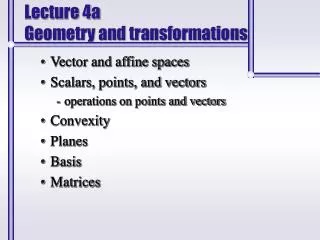
Lecture 4a Geometry and transformations. Vector and affine spaces Scalars, points, and vectors operations on points and vectors Convexity Planes Basis Matrices. Vector spaces. Scalar a real number, denoted , , , , etc. length of line seg (2m), angle of rotation (90 ) Vector

E N D
Lecture 4aGeometry and transformations • Vector and affine spaces • Scalars, points, and vectors • operations on points and vectors • Convexity • Planes • Basis • Matrices
Vector spaces • Scalar • a real number, denoted , , , , etc. • length of line seg (2m), angle of rotation (90) • Vector • a line segment with a direction and a magnitude, denoted u, v, w; u(i,j,k) • vectors have no position, but we often reference them from the origin same magnitudes diff. directions same directions diff. magnitudes same directions same magnitudes
Vector spaces • Operations that must be defined in a vector space • scalar addition and multiplication scalar • scalar-vector multiplication vector • vector-vector addition vector • there must exist a zero vector • Examples of vector spaces • geometric operations on line segments • solutions to homogeneous linear differential equations (functions can be vectors)
Affine space • Point - a position, denoted P, Q; P(x,y,z) • an affine space is a vector space plus a point • Operations that must be defined in an affine space • vector-point addition point (pt-pt sub v) • no standard addition between two points • Examples of affine spaces • geometrical operations on points • solution of linear non-homogeneous ordinary differential equations
v Q P=Q+v v=P-Q Q P w=u+v v u u v=2u Vectors • Vector-point addition P = v + Q • Point-point subtraction v = P - Q • Vector-vector addition u+v=w, where, wi = ui+vi • Vector-scalar multiplication u=v, where vi= wi P w=P-R v=P-Q R u=Q-R Q w = u+v = (P-Q)+(Q-R) = P-R
Lines • Sum of point and vector • P() = P0+v, is a point for any value of , where P0 is a point, v is a vector, is a scalar • This is the parametric form of the line • We generate points on the line by varying the parameter , usually from 0 to 1 • when =0, P()=P0 • when =1, P()=P0 + v • when =0.5, • P()=P0 + 0.5v (the midpoint) P(1)=|v| P(0.5) P(0)=P0
Affine sums • Point-point addition • If we represent a point as p=(x,y,z) and a vector as v=(i,j,k), technically there is no difference, we can add 2 points like 2 vectors • But it doesn’t make sense geometrically to add two points! • Affine addition is equivalent to parametrizing a line and can be used to generate points along a line when a line is defined by two points
P=(1.75)R+(-0.75)Q R P=(0.25)R+(0.75)Q Q P=(0.25)R+(0.75)Q Affine addition P() = P0+v P(1.75) P = Q+v P(1)= P0 +v P(0.25) v If v = R-Q, then P = Q + (R-Q) P = Q + R - Q P = R + (1-)Q P(0)=P0 P(-0.25) P = 1R + 2Q, where 1+2 = 1
Interpolation Given either P and V, or Q and R, you can generate parameters to interpolate (or extrapolate) along a line v P3=(0.75)v R P2=(0.50)v P1=(0.25)v P3=(0.75)Q + (0.25)R P P2=(0.50)Q + (0.50)R P1=(0.25)Q + (0.75)R Q
Convexity • Convex object An object for which any point lying on a line segment connecting any two points in the object is also in the object. P1 R P2 P Q P1 P2 convex (trivially) not convex convex
R P() Q P() R P() P() Q S Convexity • Constraining the alphas to sum to 1 constrains the space of points • P = 1R + 2Q, where 1+2=1 (constrains P to lie on line RQ) • P = 1R + 2Q + 3S, where 1+2+3=1 (constrains P to lie on the plane RQS)
R P() P() Q Q Convexity • Convex hull If we add the extra constraint that must be between 0 and 1, it constrains all points to lie inside the object R S line segment 0<= 1,2<=1 P=1R+2Q planar polygon 0<= 1-n<=1 P=1P1+2P2+...+nPn triangle 0<= 1,2,3<=1 P=1R+2Q +3S
Dot product • The dot, or inner, product is uv = u1v1 + u2v2 + u3v3 for u = (u1,u2,u3) and v = (v1,v2,v3) • The dot product is a scalar value equal to the • a. magnitude of (vector x projected onto vector y) • b. cosine of angle between the normalized vectors • properties: If uv=0, u and v are orthogonal (*) |u|2 =uu, the square of the magnitude (*)
y u u =90 v v x Dot product if u,v normalized, |u|=|v|=1, cos=uv cos(90)=0, cos(0)=1 u,v orthogonal cos=uv /|u||v| uv = 0
a b c Cross product • The cross product of two vectors is u x v = | u2v3 - u3v2 | = w | u3v1 - u1v3 | | u1v2 - u2v1 | • The cross product is a vector and gives a normal to the plane defined by vectors a and b • properties: |sin| = u x v / |u||v| w is orthogonal to both u and v: a c = 0 b c = 0 c is the green vector coming out of the screen - use the right hand rule to find c
u P0 v Planes • Parametric • T(,) = P0 + u + v • choose parameters to find a point on the plane • good for generating points on a plane what happens when we constrain and to be between 0 and 1?
n u P0 v P Planes • Normal (implicit) • (P - P0) n = 0, where n = u x v • if you have a P that satisfies, then it’s on plane, but this doesn’t tell you how to find it • good for testing to see if point is a plane (P - P0) n = 0 P n = P0 n [x y z][abc]T = d ax+by+ cz= d
P3 P0 P2 P1 Planes • Affine • A(1, 2, 3) = 1 P1 +2 P2 +3 P3 , where 1 +2 +3 = 1 • a third form • a reformulation of parametric form
Coordinate system and frame • Coordinate space • in a vector space, vectors aren’t unique • the vectors u and v are the same in both cases: • Frame • because an affine space contains points, we can ‘fix’ the vectors at some point • a frame is a coord. system with an origin • (typically, no distinction is made and I will use the two terms synonymously) u v u v
Basis • Draw vector w = (3,4,2) w = 3x + 4y + 2z = (3,0,0) + (0,4,0) + (0,0,2) = (3,4,2) Notice that w contains some component of x, some of y, and some of z. x, y, and z are the basis vectors of w
1 a = 2 3 v1 w = aT v2 v3 Basis • We can represent any vector in terms of three linearly independent vectors as w = 1v1 + 2v2 + 3v3 • scalars 1 2 3 are the components of w w.r.t. basis vectors v1 v2 v3 • we can represent w w.r.t. this basis as a matrix Text convention: boldface means basis is implied* OR aT = [1 2 3 ]
3 a = 4 2 x w = aT y z Example • Go through example use vector w = (3,4,2) now add vectors u and v to create another basis • these vectors are orthogonal • (how did I create them?)
Normalizing vectors • Normalized, or unit vectors • have a magnitude of 1 • have a direction equal to the original • most of the time we will use the normalized form of the vector • keep magnitude around - it may be needed if w = ax + by + cz then, wUNIT = (ax + by + cz) / sqrt(a*a + b*b + c*c)
v1 M v2 v3 u1 u2 u3 a b c d e f g h i M = Matrices • A matrix is simply an array of numbers. • We can represent a system of vectors as a matrix, M u1 = av1 + bv2 + cv3 u2 = dv1 + ev2 + fv3 u3 = gv1 + hv2 + iv3 u is defined in terms of v OR =
m m m = C A + B = A+B n n n Aij + Bij where Cij = Matrices - addition • Matrix addition If A is nxm and B is nxm, then A+B is also nxm A and B are conformalfor addition if A and B have the same dimensions
m m k = C = A B AB n n k kr=1 Air Brj where Cij = Matrices - multiplication • Matrix multiplication If A is nxk and B is kxm, then AB is nxm rows of A x cols of B A and B are conformalfor multiplication if the no. of columns of A equals the no. of rows of B
1 0 0 0 1 0 0 0 1 I= Matrix properties • A+B = B+A addition is commutative • A+(B+C) = (A+B)+C addition is associative • A(BC) = (AB)C multiplication is associative • AB = BA multiplication is NOT commutative • (in general; some special cases are) • AI = IA = A A times the identity matrix is A, • where, the identity matrix is a • square matrix (nxn) that has ones • along the diagonal
y x z 1 m m = 1 x y xyT k k Vector properties • The dot product or inner product is • xTy = xy = • The inner product is a scalar equal to • 1) the magnitude of vector x projected onto vector y • 2) the cosine of the angle between the normalized vectors • The outer product is xyT ni=1 xi yj xy = ||z||
0 -uz uy uz 0 -ux -uy ux 0 vx vy vz u x v = = n u v n Vector properties • The cross product of two vectors is • Occasionally, this form is used i j k u1 u2 -u3 -v1 v2 v3 u x v = = n n is orthogonal to both u and v: u n = 0, v n = 0 n is normal to the plane formed by u and v
Matrix properties - transpose • The transpose of a matrix is AT • where AT = [aij]T = [aji] • (A)T = AT • (the transpose of a scalar & a matrix equals the scalar times the transpose of the matrix) • (A+B)T = AT + BT • (the transpose of A+B equals the transpose of A plus the transpose of B) • (AT)T = A • (the transpose of A transpose equals A)
Matrix properties - inverse • The inverse of a matrix is A-1 • if Ax = b, then x = A-1b • A-1A = AA-1 = I • (A inverse times A equals A times A inverse, equals the Identity matrix) • (AB)-1 = B-1A-1 • (the inverse of A times B equals B inverse times A inverse) x is an mx1 matrix, or vector
Matrix properties - determinant • The determinant of a matrix is • det(A) = • The determinant is the volume (area) • of the parallelpiped (parallelogram) • defined by the column vectors of A nj=1 (-1)i+j aij det(A[ij]) nxn matrix (determinants are only defined for square matrices) the ij’th minor of A - obtained by removing the ith row and jth column of A
Determinant properties* det(A) = det(AT) det(A) = ndet(A), where A is nxn det(AB) = det(A) det(B) det(A-1) = 1/det(A)
Matrix properties • These statements are equivalent*: 1) A is singular 2) A-1 does not exist 3) There exists a non-zero vector x such that Ax = 0 4) det(A) = 0 (*where A is a square matrix)