Download
1 / 26
260 likes | 373 Views
Solving POMDPs Using Quadratically Constrained Linear Programs. Christopher Amato Daniel S. Bernstein Shlomo Zilberstein University of Massachusetts Amherst January 6, 2006. Overview. POMDPs and their solutions Fixing memory with controllers Previous approaches

E N D
Solving POMDPs Using Quadratically Constrained Linear Programs Christopher Amato Daniel S. Bernstein Shlomo Zilberstein University of Massachusetts Amherst January 6, 2006
Overview • POMDPs and their solutions • Fixing memory with controllers • Previous approaches • Representing the optimal controller • Some experimental results
POMDPs • Partially observable Markov decision process (POMDP) • Agent interacts with the environment • Sequential decision making under uncertainty • At each stage receives: • an observation rather than the actual state • Receives an immediate reward a Environment o,r
POMDP definition • A POMDP can be defined with the following tuple: M = S, A, P, R, , O • S, a finite set of states with designated initial state distribution b0 • A, a finite set of actions • P, the state transition model: P(s'| s, a) • R, the reward model: R(s, a) • , a finite set of observations • O, the observation model: O(o|s',a)
POMDP solutions • A policy is a mapping: W* A • Goal is to maximize expected discounted reward over an infinite horizon • Use a discount factor, , to calculate this
Example POMDP: Hallway Minimize number of steps to the starred square for a given start state distribution States: grid cells with orientation Actions: turn , , , move forward, stay Transitions: noisy Observations: red lines Goal: starred square
Previous work • Optimal algorithms • Large space requirement • Can only solve small problems • Approximation algorithms • provide weak optimality guarantees, if any
Policies as controllers • Fixed memory • Randomness used to offset memory limitations • Action selection, ψ : Q →A • Transitions, η : Q × A × O →Q • Value given by Bellman equation:
Controller example • Stochastic controller • 2 nodes, 2 actions, 2 obs • Parameters • P(a|q) • P(q’|q,a,o) o1 a1 o2 a2 o2 0.25 0.75 0.5 0.5 1.0 1.0 1 2 1.0 1.0 o1 1.0 a1 o2
Optimal controllers • How do we set the parameters of the controller? • Deterministic controllers - traditional methods such as branch and bound (Meuleau et al. 99) • Stochastic controllers - continuous optimization
Gradient ascent • Gradient ascent (GA)- Meuleau et al. 99 • Create cross-product MDP from POMDP and controller • Matrix operations then allow a gradient to be calculated
Problems with GA • Incomplete gradient calculation • Computationally challenging • Locally optimal
BPI • Bounded Policy Iteration (BPI) - Poupart & Boutilier 03 • Alternates between improvement and evaluation until convergence • Improvement: For each node, find a probability distribution over one-step lookahead values that is greater than the current node’s value for all states • Evaluation: Finds values of all nodes in all states
BPI - Linear program For a given node, q Variables: x(a)= P(a|q), x(q’,a,o)=P(q’,a|q,o) Objective: Maximize Improvement Constraints: s S Probability constraints: a A Also, all probabilities must sum to 1 and be greater than 0
Problems with BPI • Difficult to improve value for all states • May require more nodes for a given start state • Linear program (one step lookahead) results in local optimality • Must add nodes when stuck
QCLP optimization • Quadratically constrained linear program (QCLP) • Consider node value as a variable • Improvement and evaluation all in one step • Add constraints to maintain valid values
QCLP intuition • Value variable allows improvement and evaluation at the same time (infinite lookahead) • While iterative process of BPI can “get stuck” the QCLP provides the globally optimal solution
QCLP representation Variables: x(q’,a,q,o) = P(q’,a|q,o), y(q,s)= V(q,s) Objective: Maximize Value Constraints: s S, q Q Probability constraints: q Q, a A, o Ω Also, all probabilities must sum to 1 and be greater than 0
Optimality Theorem: An optimal solution of the QCLP results in an optimal stochastic controller for the given size and initial state distribution.
Pros and cons of QCLP • Pros • Retains fixed memory and efficient policy representation • Represents optimal policy for given size • Takes advantage of known start state • Cons • Difficult to solve optimally
Experiments • Nonlinear programming algorithm (snopt) - sequential quadratic programming (SQP) • Guarantees locally optimal solution • NEOS server • 10 random initial controllers for a range of sizes • Compare the QCLP with BPI
Results (a) best and (b) mean results of the QCLP and BPI on the hallway domain (57 states, 21 obs, 5 acts) (a) (b)
Results (a) (b) (a) best and (b) mean results of the QCLP and BPI on the machine maintenance domain (256 states, 16 obs, 4 acts)
Results • Computation time is comparable to BPI • Increase as controller size grows offset by better performance Hallway Machine
Conclusion • Introduced new fixed-size optimal representation • Showed consistent improvement over BPI with a locally optimal solver • In general, the QCLP may allow small optimal controllers to be found • Also, may provide concise near-optimal approximations of large controllers
Future Work • Investigate more specialized solution techniques for QCLP formulation • Greater experimentation and comparison with other methods • Extension to the multiagent case