Based on customer demand, estimate: ω s : minimum required amount of material s

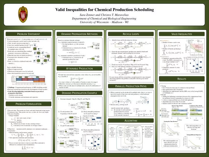
1. Feed A Valid Inequalities for Chemical Production Scheduling Heat Backward Propagation Product 1 Step 3 Step 0 Step 1 Step 2 Set ωs = 0 for tear states, calculate ωs for products, and set n = 0 Set Ik= ∅ and Sk = {products & tear states} Calculate μiand then μi*∀i∉Iks.t. Si+\Sk = ∅. Add these tasks to Ik Calculate ωs∀s∉(Sk\ST ) s.t. Is-\Ik = ∅. Add these states to Sk 40% Int AB 40% 10% React2 Capacity: U1 20-25 kg, U2 45-50 kg Capacity: U1 20-25 kg, U2 45-50 kg 60% • U1U2 • 0 0 • 0 1 • 0 2 • 1 0 • 1 • 20 • 21 • 30 • U1U2 • 0 0 • 0 1 • 0 2 • 1 0 • 1 • 20 • 21 • 30 Sara Zenner and Christos T. Maravelias Department of Chemical and Biological Engineering University of Wisconsin – Madison - WI Hot A S3 10% T3 Capacity: U3 30-40kg 60% T1= 55 →T1* = 60 Impure E *= 60 →̂= 75 3 2 1 Separate 90% Int BC # of Batches T1 T2 90% Does Ik=I & Sk=S? S1 S4 S2 # of Batches # of Batches T3=50→T3* =60 No 50% React3 React1 Product 2 80% Feed B 0 20 40 60 80 100 120 20% 50% Yes Feed C Is n≥ |ST|? No Yes 0 0 20 20 40 40 60 60 80 80 100 100 Set n = n+1 Stop Update Tear Streams Problem Statement Demand Propagation Methods Recycle Loops Valid Inequalities • Given are a set of tasks iI, processing units jJ, and materials sS • A processing unit j can be used to carry out tasks iIj. • Task i in unit j has processing time τij • Unit j has variable batchsize in [βjmin,βjmax] • A material can be consumed/produced • by multiple tasksiIs-/iIs+. • Each task can consume/produce multiple • materials; conversion coefficient ριs • Materials may have an initial inventory ζs • Customers have demands for final • products ϕst • State s is stored in a dedicated tank with • capacity γs • Find a schedule showing: • When to begin each task • Which processing unit to use for each task • How much material to process for each task • Challenge: Computational performance of MIP scheduling models • Previous research has focused on the development of better models • Goal: Develop tightening constraints based on specialized propagation algorithms • Include recycle streams • Consider minimum and maximum unit capacities • Based on customer demand, estimate: • ωs: minimum required amount of material s • For final products, ωsis the customer demand • Calculated once µi is known for all tasks consuming material s • μi: minimum cumulative production of task i • Calculated once ωs is known for all materials produced by task i Identify loops and break using tear streams Guess the tear stream doesn’t produce any material; backward propagate demand until reaching the tear stream Check tear stream: T3 produces 50kg of S5, but T4 needs 52kg Start over with updated cumulative production for S5 If a tear stream still does not produce enough material to meet demand after being updated, the problem is infeasible with the given initial inventories • Constraint 1 • Number of times a task is run • Number of batches producing a state • Constraint 2 • Cumulative amount produced by a task. The RHS is increased so it is an integer multiple of βjmax • Cumulative amount of a state produced 50% 50% 50% 50% T2: 40 T2 T2: 40 T2: 40 15 15 15 15 S4 S4 S4 S4 S1 S1 S1 S1 S3 S3 S3 S3 50% 50% 50% 50% 20 20 S5 S5 S5 S5 20 20 T1 T1 T1: 60 T1 55 55 10% 25% 25% 25% 25% T3: 60 T3: 60 T3 T3: 60 50 50 50 50 S6 S6 S6 S6 90% {U1,U2} {U1,U2} {U1,U2} {U1,U2} T1 T2 T3 75% 75% 75% 75% How much? S2 S2 S2 S2 {U3} {U3} {U3} {U3} S1 S2 S3 S4 Where? Heater Heat/52 Heat/20 Heat/48 Heater React1/50 React2/50 React1/50 React2/50 React2/50 Reactor 1 T2= 40 is attainable Reactor 2 React3/80 React3/55 React2/70 React1/80 React2/80 Separator T1= 55 Separator Separate/80 Separate/55 Reactors 1&2 When? 0 1 2 3 4 5 7 8 9 10 6 Attainable Production Amount Produced Amount Produced Amount Produced • If units have min and max capacities, some values of μi are not feasible • μi is feasible if • for some k, whereαjk is the number of batches in unit j for range k. • Otherwise, increase i to the nearest attainable amount i* ≥ i • When a task can take place in multiple units, check all combinations of batches in units Results Tighter Formulation Original Formulation • Testing • Test 36 discrete-time and 12 continuous-time problems • Stop optimization after 30 minutes • Algorithm was implemented and the MIPs were solved using GAMS 23.7/CPLEX 12.3 • Results • Adding the tightening constraints decreases the computational time for problems solved to optimality by a factor of >100 • > twice as many problems are solved with tightening • Algorithm runs in less than 10 seconds • Similar results for discrete and continuous models Parallel Production Paths • When a material can be produced by multiple tasks, there is no way to know how much of that state each task produces, so the backward propagation does not work • Instead, find i solving an LP: • min the amount task i produces • s.t. the amount of each material s • produced must be at least:(1) ωs (when ωs is known), and • (2) the amount consumed Demand Propagation Example S2 S2 S2 S4 S4 S4 S1 S1 S1 S3 S3 S3 50-150 50-150 50-150 50-150 50-150 50-150 55-90 55-90 55-90 • Customer demand: 15kg S4, 20kg S5, and 50kg S6 • 2a. T3 only produces S6; 2b. Check attainable production • T2 produces both S4 and S5 for T2 and T3 to find μ* • T2 and T3 both need S3 • 4b. Check attainable production for T1 to find μ* • 4a. T1 produces S5 50% 50% 50% φS4= 50 φS4= 50 φS4= 50 T1 T1: 110 T1: 110 T2: 100 T2 T2: 104 T3: 100 T3: 104 T3 65 100 100 50 65 104 104 50 ζS1= 45 ζS1= 45 ζS1= 45 50-150 50-150 50-150 50% 50% 50% 80% 80% 80% T4: 65 T4: 65 T4 52 52 20% 20% 20% S5 S5 S5 S6 S6 S6 Problem Formulation 50% 50% T1: 50 ω= 55 T2: 30 • Discrete time: Time points are fixed, and tasks begin/end at time points • Continuous time: Time points can vary, so tasks can have any length • Decision Variables: • Integer Variable: • Continuous Variables: • Bijt = Batch size of task i in unit j starting at time t • Sst= Inventory level of material s in storage at time t • Objectives: maximize profit, minimize cost, minimize makespan, … • Constraints: • Material balance and inventory capacity • Unit capacities (minimum and maximum) • Process at most one task at a time in a unit (This constraint is different for continuous time formulations) 20% 20 μ= 100 80% 50 Algorithm Varying the Time Horizon The valid inequalities are effective for long time horizons Ik: Tasks for which μi is known Sk: States for which ωs is known ST: set of tear states n: number of times tear stream has been updated Testing Different Objectives Discrete Time Model (Shah et al., 1993) Continuous Time Model (Sundaramoorthy and Karimi, 2005) Solved to Optimality (avg. CPU time) No Tightening No Tightening 2.1% 189 s 1.3% 149 s 2.2% The valid inequalities are more effective for cost minimization than for makespan minimization With Tightening With Tightening 1.5% T3=50 Not Solved to Optimality (avg. optimality gap) 1.4 s 2.4 s 0.45 s 41.2 s 0 14 34 36 0 6 12 Problems Problems