Download
1 / 26
260 likes | 749 Views
Chapter 4: Induction and Recursion. Discrete Mathematics and Its Applications. Lingma Acheson (linglu@iupui.edu) Department of Computer and Information Science, IUPUI. 4.1 Mathematical Induction. Introduction.

E N D
Chapter 4: Induction and Recursion Discrete Mathematics and Its Applications Lingma Acheson (linglu@iupui.edu) Department of Computer and Information Science, IUPUI
4.1 Mathematical Induction Introduction • Mathematical Induction is used to show that P(n) is true for every positive integer n. • Used only to prove results obtained in some other way. • Example: Suppose we have an infinite ladder, and we want to know whether we can reach every step on the ladder. We know two things 1. We can reach the first rung of the ladder. 2. If we can reach a particular rung of the ladder, then we can reach the next rung. Can we conclude that we can reach every rung? By 1, we can reach the first rung. By 2, we can reach the second rung. Apply 2 again, we can reach the third rung… After 100 uses of 2, we can reach the 101st rung….
4.1 Mathematical Induction To complete the inductive step of a proof using the principle of mathematical induction, we assume that P(k) is true for an arbitrary positive integer k and show that under this assumption, P(k+1) must also be true. The assumption that P(k) is true is called the inductive hypothesis. The proof technique is stated as [P(1)Λk(P(k) →P(k+1) )] → nP(n) where the domain is the set of positive integers Mathematical Induction PRINCIPLE OF MATHEMATICAL INDUCTION To prove that P(n) is true for all positive integers n, where P(n) is a propositional function, we complete two steps. BASIS STEP: We verify that P(1) is true. INDUCTIVE STEP: We show that the conditional statement P(k) →P(k+1) is true for all positive integers k. 3
4.1 Mathematical Induction Show that if n is a positive integer, then Solution: BASIS STEP: P(1) is true, because 1 = INDUCTIVE STEP: For the inductive hypothesis we assume that P(k) holds for an arbitrary positive integer k. That is, we assume that Under this assumption, it must be shown that P(k+1) is true, i.e.: When we add k+1 to both sides of the equation in P(k), we obtain This shows that P(k+1) is true under the assumption that P(k) is true. This complete the inductive step. Examples of Proofs by Mathematical Induction 4
4.1 Mathematical Induction Use mathematical induction to prove that n3 – n is divisible by 3 whenever n is a positive integer. Solution: BASIS STEP: The statement P(1) is true because 13 – 1 = 0 is divisible by 3. INDUCTIVE STEP: For the inductive hypothesis we assume that P(k) is true; that is we assume that k3 – k is divisible by 3. To complete the inductive step, we must show that when we assume the inductive hypothesis, the statement (k+1)3 – (k+1) is also divisible by 3. (k+1)3 – (k+1) = (k3 + 3k2 + 3k + 1) – (k + 1) = (k3 – k) + 3(k2 + k) By inductive hypothesis, we know that (k3 – k) is divisible by 3; and the second term is also divisible by 3. This completes the inductive step. 5
4.3 Recursive Definitions and Structural Induction Introduction 6
4.3 Recursive Definitions and Structural Induction Sometimes it’s easier to define an object in terms of itself. This process is called Recursion. Example: the sequence of powers of 2 is given by an = 2n for n = 0, 1, 2, …. This sequence can also be defined by giving the first term of the sequence, namely, a0 = 1, and a rule finding a term of the sequence from the previous one, namely, an+1 = 2an, for n = 0, 1, 2, …. 7
4.3 Recursive Definitions and Structural Induction Use two steps to define a function with the set of nonnegative integers as its domain: BASIS STEP: Specify that value of the function at zero. RECURSIVE STEP: Give a rule for finding its value at an integer from its values at smaller integers. Such a definition is called a recursive or inductive definition. Examples: Suppose that f is defined recursively by f(0) = 3, f(n+1) = 2f(n) + 3 Find f(1), f(2), f(3), and f(4). Solution: f(1) = 2f(0) + 3 = 2*3 + 3 = 9 f(2) = 2f(1) + 3 = 2*9 + 3 = 21 f(3) = 2f(2) + 3 = 2*21 + 3 = 45 f(4) = 2f(3) + 3 = 2*45 + 3 = 93 Recursively Defined Functions 8
4.3 Recursive Definitions and Structural Induction Examples: Give an inductive definition of the factorial function F(n) = n!. Solution: Basis Step: F(0) = 1 Inductive Step: F(n+1) = (n+1)F(n) E.g. Find F(5). F(5) = 5F(4) = 5*4F(3) = 5*4*3F(2) = 5 * 4 * 3 * 2F(1) = 5 * 4 * 3 * 2 * 1F(0) = 5 * 4 * 3 * 2 * 1 * 1 = 120 Give a recursive definition of . Solution: Basis Step: Inductive Step: 9
Example: Find the Fibonacci numbers f2, f3, f4, f5, and f6. Solution: f2 = f1 + f0 = 1 + 0 = 1, f3 = f2 + f1 = 1 + 1 = 2, f4 = f3 + f2 = 2 + 1 = 3, f5 = f4 + f3 = 3 + 2 = 5, f6 = f5+ f4 + 5 + 3 = 8. Example: Find the Fibonacci numbers f7. Solution ? 4.3 Recursive Definitions and Structural Induction DEFINITION 1 The Fibonacci numbers, f0, f1, f2, …, are defined by the equations f0= 0, f1 = 1, and fn = fn-1 + fn-2 for n = 2, 3, 4, …. 10
The basis step of the recursive definition of strings says that the empty string belongs to ∑*. The recursive step states that new strings are produced by adding a symbol from ∑ to the end of strings in ∑*. At each application of the recursive step, strings containing one additional symbol are generated. Example: If ∑ = {0,1}, the strings found to be in ∑*, the set of all bit strings are λ, specified to be in ∑* in the basis step, 0 and 1 formed during the first application of the recursive step, 00, 01, 10, and 11 formed during the second application of the recursive step, and so on. 4.3 Recursive Definitions and Structural Induction Recursively Defined Sets and Structures DEFINITION 2 The set ∑* of strings over the alphabet ∑ can be defined recursively by BASIS STEP: λ ∑* (where λ is the empty string containing no symbols). RECURSIVE STEP: If w ∑* and x ∑* , then wx ∑*. 11
Example: Well-Formed Formulae for Compound Statement Forms. We can define the set of well-formed formulae for compound statement forms involving T, F, propositional variables, and operators from the set {¬, Λ, V, →, ↔}. BASIS STEP: T, F, and s, where s is a propositional variable, are well-formed formulae. RECURSIVE STEP: If E and F are well-formed formulae, then (¬E), (E ΛF), (E V F), (E → F), and (E ↔ F) are well-formed formulae. By the basis step we know that T, F, p, and q are well-formed formulae, where p and q are propositional variables. From an initial application of the recursive step, we know that (p V q), (p → F), (F → q), and (qΛF) are well-formed formulae. A second application of the recursive step shows that ((p V q) → (qΛF)), (q V (p V q)), and ((p → F) → T) are well-formed formulae. 4.3 Recursive Definitions and Structural Induction 12
4.3 Recursive Definitions and Structural Induction DEFINITION 4 The set of rooted trees, where a rooted tree consists of a set of vertices containing a distinguished vertex called the root, and edges connecting these vertices, can be defined recursively by these steps: BASIS STEP: A single vertex r is a rooted tree. RECURSIVE STEP: Suppose that T1, T2, …, Tn are disjoint rooted trees with roots r1, r2, …, rn, respectively. Then the graph formed by starting with a root r, which is not in any of the rooted trees, T1, T2, …, Tn, and adding an edge from r to each of the vertices r1, r2, .., rn, is also a rooted tree. 13
4.3 Recursive Definitions and Structural Induction DEFINITION 5 The set of extended binary trees can be defined recursively by these steps: BASIS STEP: The empty set is an extended binary tree. RECURSIVE STEP: IfT1 and T2 are disjoint extended binary trees, there is an extended binary tree, denoted by T1 ·T2 , consisting of a root r together with edges connecting the root to each of the roots of the left subtree T1and the right subtree T2 when these trees are nonempty. 15
4.3 Recursive Definitions and Structural Induction DEFINITION 6 The set of full binary trees can be defined recursively by these steps: BASIS STEP: There is a full binary tree consisting only of a single vertex r. RECURSIVE STEP: IfT1 and T2 are disjoint full binary trees, there is full binary tree, denoted by T1 ·T2 , consisting of a root r together with edges connecting the root to each of the roots of the left subtree T1and the right subtree T2. 17
Example: Give a recursive algorithm for computer n!, when n is a nonnegative integer. Review: Basis Step: F(0) = 1 Inductive Step: F(n+1) = (n+1)F(n) E.g. Find F(5). F(5) = 5F(4) = 5*4F(3) = 5*4*3F(2) = 5 * 4 * 3 * 2F(1) = 5 * 4 * 3 * 2 * 1F(0) = 5 * 4 * 3 * 2 * 1 * 1 = 120 4.4 Recursive Algorithms Introduction DEFINITION 1 An algorithm is called recursive if it solves a problem by reducing it to an instance of the same problem with smaller input. ALGORITHM 1 A Recursive Algorithm for Computing n!. procedure factorial(n: nonnegative integer) if n = 0 then factorial(n):=1 else factorial(n):=n*factorial(n-1) 19
Example: Give a recursive algorithm for computer an, where a is a nonzero number and n is a nonnegative integer 4.4 Recursive Algorithms ALGORITHM 2 A Recursive Algorithm for Computing an. procedure power(a: nonzero real number, n: nonnegative integer) if n = 0 then power(a,n):=1 else power(a,n):=a*power(a, n-1) 20
Example: Express the linear search algorithm as a recursive procedure. 4.4 Recursive Algorithms ALGORITHM 5 A Recursive Linear Search Algorithm. procedure search(i,j,x: i,j,x integers, 1 <=i<=n, 1<=j<=n) if ai = x then location := i else if i = j then location : = 0 else search(i+1,j, x) 21
Example: Construct a recursive version of a binary search algorithm 4.4 Recursive Algorithms ALGORITHM 6 A Recursive Binary Search Algorithm. procedure binarySearch(i,j,x: i,j,x integers, 1 <= i <= n, 1<= j <= n) m := if x = am then location := m else if (x < am and i < m ) then binarySearch(x, i, m-1) else if (x > am and j > m ) then binarySearch(x, m+1, j) else location := 0 22
Sometimes we start with the value of the computation at one or more integers, the base cases, and successively apply the recursive definition to find the values of the function at successive larger integers. Such a procedure is called iterative. How many additions are performed to find fibonacci(n)? 4.4 Recursive Algorithms Recursion and Iteration ALGORITHM 7 A Recursive Algorithm for Fibonacci Numbers. procedure fibonacci(n: nonnegative integer) if n = 0 then fibonacci(0) := 0 else if (n = 1) then fibonacci(1) := 1 else fibonacci(n) := fibonacci(n-1) + fibonacci(n-2) 23
4.4 Recursive Algorithms f4 f3 f2 fn+1 -1 addition to find fn f2 f0 f1 f1 f0 f1 24
How many additions are performed to find fibonacci(n)? 4.4 Recursive Algorithms ALGORITHM 8 An Iterative Algorithm for Computing Fibonacci Numbers. procedure iterativeFibonacci(n: nonnegative integer) if n = 0 then y:= 0 else begin x := 0 y := 1 for i := 1 to n -1 begin z := x + y x : = y y : = z end end {y is the nth Fibonacci number} 25 n – 1 additions are used for an iterative algorithm.
Java demo for two algorithms Recursive algorithm may require far more computation than an iterative one. Sometimes it’s preferable to use a recursive procedure even if it is less efficient. Sometimes an iterative approach is preferable. 4.4 Recursive Algorithms 26