Download
1 / 33
330 likes | 444 Views
The dynamic nature of the proteome. The proteome of the cell is changing Various extra-cellular, and other signals activate pathways of proteins. A key mechanism of protein activation is post-translational modification (PTM) These pathways may lead to other genes being switched on or off

E N D
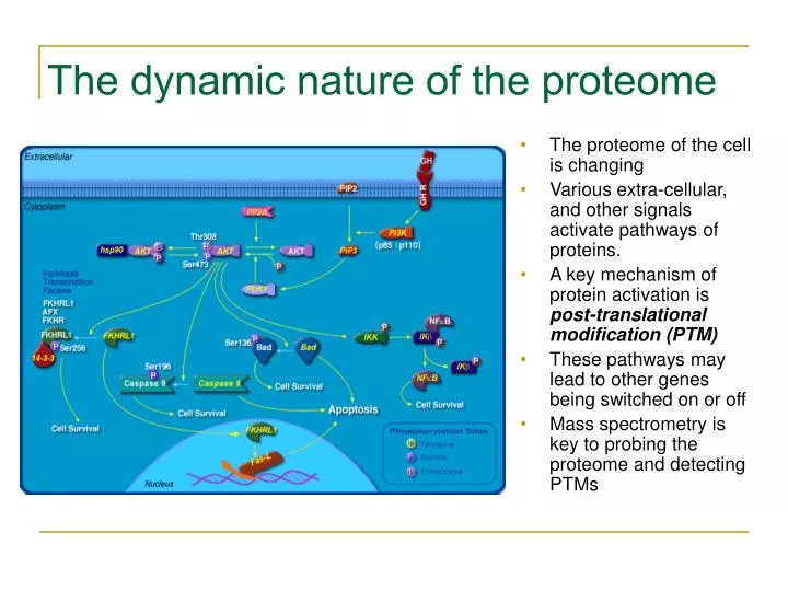
The dynamic nature of the proteome • The proteome of the cell is changing • Various extra-cellular, and other signals activate pathways of proteins. • A key mechanism of protein activation is post-translational modification (PTM) • These pathways may lead to other genes being switched on or off • Mass spectrometry is key to probing the proteome and detecting PTMs
Post-Translational Modifications Proteins are involved in cellular signaling and metabolic regulation. They are subject to a large number of biological modifications. Almost all protein sequences are post-translationally modified and 200 types of modifications of amino acid residues are known.
Examples of Post-Translational Modification Post-translational modifications increase the number of “letters” in amino acid alphabet and lead to a combinatorial explosion in both database search and de novo approaches.
Search for Modified Peptides: Virtual Database Approach Yates et al.,1995: an exhaustive search in a virtual database of all modified peptides. Exhaustive search leads to a large combinatorial problem, even for a small set of modifications types. Problem (Yates et al.,1995). Extend the virtual database approach to a large set of modifications.
Phosphorylation? Exhaustive Search for modified peptides. • YFDSTDYNMAK • 25=32 possibilities, with 2 types of modifications! Oxidation? • For each peptide, generate all modifications. • Score each modification.
Peptide Identification Problem Revisited Goal: Find a peptide from the database with maximal match between an experimental and theoretical spectrum. Input: • S: experimental spectrum • database of peptides • Δ: set of possible ion types • m: parent mass Output: • A peptide of mass m from the databasewhose theoretical spectrum matches the experimental S spectrum the best
Modified Peptide Identification Problem Goal: Find a modified peptide from the database with maximal match between an experimental and theoretical spectrum. Input: • S: experimental spectrum • database of peptides • Δ: set of possible ion types • m: parent mass • Parameter k(# of mutations/modifications) Output: • A peptide of mass m that is at most k mutations/modifications apart from a database peptide and whose theoretical spectrum matches the experimental S spectrum the best
Database Search: Sequence Analysis vs. MS/MS Analysis Sequence analysis: similar peptides (that a few mutations apart) have similar sequences MS/MS analysis: similar peptides (that a few mutations apart) have dissimilar spectra
Peptide Identification Problem: Challenge Very similar peptides may have very different spectra! Goal: Define a notion of spectral similarity that correlates well with the sequence similarity. If peptides are a few mutations/modifications apart, the spectral similarity between their spectra should be high.
Deficiency of the Shared Peaks Count Shared peaks count (SPC): intuitive measure of spectral similarity. Problem: SPC diminishes very quickly as the number of mutations increases. Only a small portion of correlations between the spectra of mutated peptides is captured by SPC.
SPC Diminishes Quickly no mutations SPC=10 1 mutation SPC=5 2 mutations SPC=2 S(PRTEIN) = {98, 133, 246, 254, 355, 375, 476, 484, 597, 632} S(PRTEYN) = {98, 133, 254, 296, 355, 425, 484, 526, 647, 682} S(PGTEYN) = {98, 133, 155, 256, 296, 385, 425, 526, 548, 583}
Elements of S2 S1represented as elements of a difference matrix. The elements with multiplicity >2 are colored; the elements with multiplicity =2 are circled. The SPC takes into account only the red entries
Spectral Convolution: An Example 5 4 3 Spectral Convolution 2 1 0 -150 -100 -50 0 50 100 150 x
Spectral Comparison: Difficult Case S = {10, 20, 30, 40, 50, 60, 70, 80, 90, 100} Which of the spectra S’ = {10, 20, 30, 40, 50, 55, 65, 75,85, 95} or S” = {10, 15, 30, 35, 50, 55, 70, 75, 90, 95} fits the spectrum S the best? SPC: both S’ and S” have 5 peaks in common with S. Spectral Convolution: reveals the peaks at 0 and 5.
Spectral Comparison: Difficult Case S S’ S S’’
Limitations of the Spectrum Convolutions Spectral convolution does not reveal that spectra S and S’ are similar, while spectra S and S” are not. Clumps of shared peaks: the matching positions in S’ come in clumps while the matching positions in S” don't. This important property was not captured by spectral convolution.
Shifts A = {a1 < … < an} : an ordered set of natural numbers. A shift (i,) is characterized by two parameters, the position (i) and the length (). The shift (i,) transforms {a1, …., an} into {a1, ….,ai-1,ai+,…,an+ }
Shifts: An Example The shift (i,) transforms {a1, …., an} into {a1, ….,ai-1,ai+,…,an+ } e.g. 10 20 30 40 50 60 70 80 90 10 20 30 35 45 55 65 75 85 10 20 30 35 45 5562 72 82 shift (4, -5) shift (7,-3)
Spectral Alignment Problem • Find a series of k shifts that make the sets A={a1, …., an} and B={b1,….,bn} as similar as possible. • k-similarity between sets • D(k) - the maximum number of elements in common between sets after k shifts.
Representing Spectra in 0-1 Alphabet • Convert spectrum to a 0-1 string with 1s corresponding to the positions of the peaks.
Comparing Spectra=Comparing 0-1 Strings • A modification with positive offset corresponds to inserting a block of 0s • A modification with negative offset corresponds to deleting a block of 0s • Comparison of theoretical and experimental spectra (represented as 0-1 strings) corresponds to a (somewhat unusual) edit distance/alignment problem where elementary edit operations are insertions/deletions of blocks of 0s • Use sequence alignment algorithms!
Spectral Alignment vs. Sequence Alignment • Manhattan-like graph with different alphabet and scoring. • Movement can be diagonal (matching masses) or horizontal/vertical (insertions/deletions corresponding to PTMs). • At most k horizontal/vertical moves.
10 20 30 40 50 55 65 75 85 95 1 1 1 1 1 1 1 1 1 1 1 1 1 1 1 1 1 1 1 1 1 1 1 1 1 1 1 1 1 1 1 1 1 1 1 1 1 1 1 1 1 1 1 1 1 1 1 1 1 1 1 1 1 1 1 1 1 1 1 1 1 1 1 1 1 1 1 1 1 1 1 1 1 1 1 1 1 1 1 1 1 1 1 1 1 1 1 1 1 1 1 1 1 1 1 1 1 1 1 1 Spectral Product A={a1, …., an} and B={b1,…., bn} Spectral product AB: two-dimensional matrix with nm 1scorresponding to all pairs of indices (ai,bj) and remaining elements being 0s. SPC: the number of 1s at the main diagonal. -shifted SPC: the number of 1s on the diagonal (i,i+ )
Spectral Alignment: k-similarity k-similarity between spectra: the maximum number of 1s on a path through this graph that uses at most k+1 diagonals. k-optimal spectral alignment = a path. The spectral alignment allows one to detect more and more subtle similarities between spectra by increasing k.
Use of k-Similarity SPC reveals only D(0)=3 matching peaks. Spectral Alignment reveals more hidden similarities between spectra: D(1)=5 and D(2)=8 and detects corresponding mutations.
Black line represent the path for k=0 Red lines represent the path for k=1 Blue lines (right) represents the path for k=2
10 20 30 40 50 55 65 75 85 95 10 15 30 35 50 55 70 75 90 95 10 10 20 20 30 30 40 40 50 50 60 60 70 70 80 80 90 90 100 100 Spectral Convolution’ Limitation The spectral convolution considers diagonals separately without combining them into feasible mutation scenarios. D(1) =10 shift function score = 10 D(1) =6
Dynamic Programming for Spectral Alignment Dij(k): the maximum number of 1s on a path to (ai,bj) that uses at most k+1 diagonals. Running time: O(n4 k)
Edit Graph for Fast Spectral Alignment diag(i,j) – the position of previous 1 on the same diagonal as (i,j)
Fast Spectral Alignment Algorithm Running time: O(n2 k)
Spectral Alignment: Complications Spectra are combinations of an increasing (N-terminal ions) and a decreasing (C-terminal ions) number series. These series form two diagonals in the spectral product, the main diagonal and the perpendicular diagonal. The described algorithm deals with the main diagonal only.
Spectral Alignment: Complications • Simultaneous analysis of N- and C-terminal ions • Taking into account the intensities and charges • Analysis of minor ions