Download
1 / 34
340 likes | 447 Views
Hypoxia in Narragansett Bay Workshop Oct 2006. Dan Codiga, Jim Kremer, Mark Brush, Chris Kincaid, Deanna Bergondo . “Modeling” In the Narragansett Bay CHRP Project. Does the word “Model” have meaning?. Hydrodynamic Ecological Research vs Applied Prognostic vs Diagnostic

E N D
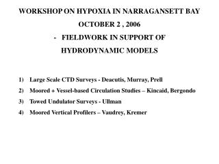
Hypoxia in Narragansett BayWorkshop Oct 2006 Dan Codiga, Jim Kremer, Mark Brush, Chris Kincaid, Deanna Bergondo “Modeling” In the Narragansett Bay CHRP Project
Does the word “Model” have meaning? • Hydrodynamic • Ecological • Research vs Applied • Prognostic vs Diagnostic • Heuristic, Theoretical, Conceptual, Empirical, Statistical, Probabilistic, Numerical, Analytic • Idealized/Process-Oriented vs Realistic • Kinematic vs Dynamic • Forecast vs hindcast
CHRP Program Goals (selected excerpts from RFP) • Predictive/modeling tools for decision makers • Models that predict susceptibility to hypoxia • Better understanding and parameterizations • Transferability of results across systems • Data to calibrate and verify models Following two presentations
Our approaches • Hybrid Ecological-Hydrodynamic Modeling • Ecological model:simple • Few processes, few parameters • Parameters that can be constrained by measurements • Few spatial domains (~20), as appropriate to measurements available • Net exchanges between spatial domains: from hydrodynamic model • Hydrodynamic model:full physics and forcing of ROMS • realistic configuration; forced by observed winds, rivers, tides, surface fluxes • Applied across entire Bay, and beyond, at high resolution • Passive tracers used to determine net exchanges between larger domains of ecological model • Empirical-Statistical Modeling • Input-output relations, emphasis on empirical fit more than mechanisms • Development of indices for stratification, hypoxia susceptibility • Learn from hindcasts, ultimately apply toward forecasting
Heuristic models in research: iterative failure = learning Processes Conceptual Model Formulations Runs that fall short Parameter values
But for management models:• Heuristic goal less impt • Accurateeven if not precise• Well constrained coefs• Simple (?) (at least understandable)_____________________________≠ Research models
25-30 state vars 70-110 params A paradox -- “Realism” = many parameters weakly constrained limited data to corroborate i.e. “Over-parameterized” (many ways to get similar results) :.Accuracy is unknown. (often unknowable)
An alternative approach? 4 state variables, 5 processes Phytoplankton O D 2 N P Processes of the model (excluding macroalgae...) Temp, Light, Boundary Conditions Chl, N, P, Salinity O2 coupled stoichiometrically Productivity Physics Surface layer - - - - - - - - - Deep layer - - - - - - - - - Bottom sediment mixing flushing Atmospheric Photic zone heterotrophy Flux to bottom deposition . N Sediment Land-use organics Benthic heterotrophy N P Denitri- fication .
Corroboration: “Strength in numbers” Shallow test sites (MA, RI, CT)
Long Island Sound -- Hypoxia August 20 Deep test sites (MA, RI, CT, VA, MD) Narragansett Bay Chesapeake Bay Long Island Sound
Hydrodynamic Model Equations Momentum balance x & y directions: u + vu – fv = f + Fu + Du t x v + vv + fu = f + Fv + Dv ty Potential temperature and salinity : T+ vT = FT + DT t S + vS = FS + DS t The equation of state: r= r (T, S, P) Vertical momentum: f = - r g z ro Continuity equation: u+v+w = 0 x y z Initial Conditions Forcing Conditions ROMS Model Regional Ocean Modeling System Output
Hydrodynamic Model Grid Resolution: 100 m Grid Size: 1024 x 512 Vertical Layers: 20 River Flow: USGS Winds: NCDC Tidal Forcing: ADCIRC Open Boundary
This project: Mid-Bay focus Narragansett Bay Commission: Providence & Seekonk Rivers Mt. Hope Bay circulation/exchange /mixing study. ADCP, tide gauges (Deleo, 2001) Extent of counter Summer, 07: 4 month deployment (Outflow pathways) Bay-RIS exchange study (98-02)
This project: Mid-Bay focus Narragansett Bay Commission: Providence & Seekonk Rivers Mt. Hope Bay circulation/exchange /mixing study. ADCP, tide gauges (Deleo, 2001) Extent of counter Summer, 08: Deep return flow processes Bay-RIS exchange study (98-02)
Model-Data Comparison Salinity - Phillipsdale Model Salinity (ppt) Data Time (days)
Hybrid: Driving Ecological model with Hydrodynamic Model: Lookup Table of Daily Exchanges (k) dP1/dt = P1(G-R) - k1,2P1V1 + k2,1P2V2 ...
Modeling Exchange Between Ecological Model Domains DYE_01 DYE_02 DYE_03 DYE_06 DYE 04 DYE 05 DYE_07 DYE_09 DYE_08
Long-term Aims:Hybrid Ecological-Physical Model • Increased spatial resolution of ecology: approach TMDL applicability • Scenario evaluation • Nutrient load changes • Climatic changes • Alternative to mechanistic coupled hydrodynamic/ecological modeling
Empirical/Statistical ModelingOverall Goals • Data-oriented—complements Hybrid– less mechanistic • Synthesize DO variability • Spatial (Large-scale CTD; towed body) • Temporal (Fixed-site buoys) • Develop indices • Stratification • Hypoxia vulnerability • First: Hindcasts to understand relationship between forcing (physical and biological) and DO responses • Long-term: Predictive capability for forecasting and scenario evaluation
Candidate predictors for DO • Biological • Chlorophyll • Temperature & solar input • Nutrient inputs (Rivers, WWTF, Estuarine exchange) • Others • Physical • River runoff, WWTF water transports • Tidal range cubed (energy available for mixing) • Windspeed cubed (energy available for mixing) • Others (Wind direction; Precip; Surface heat flux)
Strategy: start simple & develop method • Start with Bullock Reach timeseries • 5 yrs at fixed single point (no spatial information) • Investigate stratification (not DO-- yet) • Target variable: strat = [sigt(deep) – sigt(shallow)] • Include 3 candidate predictor variables: • River runoff (sum over 5 rivers) • Tidal range cubed (energy available for mixing) • Windspeed cubed (energy available for mixing)
Visually apparent features • Stratification reacts to ‘events’ in each of: • River inputs • Winds • Tidal stage • Stratification ‘events’ appear to be • Triggered irregularly by each process • Lagged by varying amounts from each process
Low-pass and subsample to 12 hrs…Compare techniques • Multiple Linear Regression (MLR) • No lags • Optimal lags – determined individually • Static Neural Network • No lags • Lags from MLR analysis • [coming soon] Dynamic Neural Network • Varying lags • Multiple interacting inputs
Observed Model Stratification Dst [kg m-3] Multiple Linear Regression No lags r2=0.42 (River alone: 0.36) MLR with lags River 2 days Wind 1 day Tide 3.5 days r2=0.51 (River alone: 0.48)
Static Neural Net No lags r2=0.55 (River alone: 0.41) Static Neural Net Lags from MLR r2=0.59 (River alone: 0.52)
Advantages/Disadvantagesof Neural Networks • Advantages • Nonlinear, can achieve better accuracy • Excels with multiple interacting predictors; • Dynamic NN: input delays capture lags • Varying lags from multiple interacting inputs • Transferable; conveniently applied to other/new data • Easy to use (surprise!!) • Main disadvantage • opaque “black-box” can be difficult to interpret; ameliorated by: complementary linear analysis, sensitivity studies, isolating/combining predictors
Next steps • Stratification • Consider additional predictors: • Surface heat flux; precipitation; WWTF volume flux • Different sites (North Prudence, etc) • Treat spatially-averaged regions • Apply similar approach to DO • Finish gathering forcing function data • Chl; solar inputs; WWTF nutrients • Corroborate Hybrid Ecological-Hydrodynamic Model