Download
1 / 93
960 likes | 1.07k Views
Introduction to Accounting. FINAL EXAM REVIEW Chapters 10,11,12, 13, 14, & 15. Standard Cost Card – Variable Production Cost. A standard cost card for one unit of product might look like this:. Standards vs. Budgets. A standard is the expected cost for one unit.

E N D
Introduction to Accounting FINAL EXAM REVIEW Chapters 10,11,12, 13, 14, & 15 A&MIS 212
Standard Cost Card – Variable Production Cost A standard cost card for one unit of product might look like this: A&MIS 212
Standards vs. Budgets • Astandardis the expected cost for one unit. • A budgetis the expected cost for all units. Are standards the same as budgets? A&MIS 212
A General Model of Variances Actual Quantity Actual Quantity Standard Quantity × × × Actual Price Standard Price Standard Price Price Variance Quantity Variance Standard price is the amount that should have been paid for the resources acquired. A&MIS 212
A General Model of Variances Actual Quantity Actual Quantity Standard Quantity × × × Actual Price Standard Price Standard Price Price Variance Quantity Variance Standard quantity is the quantity allowed for the actual good output. A&MIS 212
A General Model of Variances Actual Quantity Actual Quantity Standard Quantity × × × actual price standard price standard price Price Variance Quantity Variance AQP(ap - sp) sp(AQU - SQ) AQP = Actual Quantitysp= Standard Priceap= Actual PriceSQ = Standard Quantity A&MIS 212
Zippy Material Variances Example Hanson Inc. has the following direct material standard to manufacture one Zippy: 1.5 pounds per Zippy at $4.00 per pound Last week 1,700 pounds of material were purchased for $3.90 per pound, at total cost of $6,630, and used to make 1,000 Zippies. A&MIS 212
Material Price Variance • Based on purchases: AQP(ap - sp) = 1,700 lbs. ($3.90 - $4.00) = - $170 Favorable • Based on usage: AQU(ap - sp) = 1,700 lbs. ($3.90 - $4.00) = - $170 Favorable A&MIS 212
Material Quantity Variance Standard quantity = output sq per unit = 1,000 units 1.5 lbs./unit = 1,500 lbs. Quantity variance = (AQ – SQ) sp = (1,700 -1,500 lbs.) $4 = $800 Unfavorable A&MIS 212
Zippy Material Variances Summary Actual Quantity Actual Quantity Standard Quantity × × × Actual Price Standard Price Standard Price 1,700 lbs. 1,700 lbs. 1,500 lbs. × × × $3.90 per lb. $4.00 per lb. $4.00 per lb. =$6,630 = $ 6,800 = $6,000 Price variance$170 favorable Quantity variance$800 unfavorable A&MIS 212
Material Variances • The price variance is computed on the entire quantity purchased. • The quantity variance is computed only on the quantity used. Hanson purchased and used 1,700 pounds. How are the variances computed if the amount purchaseddiffers from the amount used? A&MIS 212
Zippy Material Variances Continued Hanson Inc. has the following material standard to manufacture one Zippy: 1.5 pounds per Zippy at $4.00 per pound Last week 2,800 pounds of material were purchased at a total cost of $10,920, and 1,700 pounds were used to make 1,000 Zippies. Compute the price variance. A&MIS 212
Zippy Actual Quantity Actual Quantity Purchased Purchased × × Actual Price Standard Price 2,800 lbs. 2,800 lbs. × × $3.90 per lb. $4.00 per lb. = $10,920 = $11,200 Price variance increases because quantity purchased increases. Price variance$280 favorable Material Variances Continued A&MIS 212
Zippy Material Variances Continued Actual Quantity Used Standard Quantity × × Standard Price Standard Price 1,700 lbs. 1,500 lbs. × × $4.00 per lb. $4.00 per lb. = $6,800 = $6,000 Quantity variance is unchanged because actual and standard quantities are unchanged. Quantity variance$800 unfavorable A&MIS 212
Zippy Labor Variances Example Hanson Inc. has the following direct labor standard to manufacture one Zippy: 1.5 standard hours per finished Zippy at $6.00 per direct labor hour Last week 1,550 direct labor hours were worked at an average cost of $6.20 per hour, for a total labor cost of $9,610, to make 1,000 Zippies. A&MIS 212
Zippy Labor Rate Variance Based on labor usage: AQ (ar - sr) = 1,550 hrs.($6.20 - $6.00) = $310 Unfavorable A&MIS 212
Zippy Labor Quantity Variance Standard quantity = output sq per unit = 1,000 units 1.5 hrs./unit = 1,500 hrs. Quantity variance = (AQ – SQ) sp = (1,550 -1,500 hrs.) $6 = $300 Unfavorable A&MIS 212
Zippy Labor Variances Summary Actual Hours Actual Hours Standard Hours × × × Actual Rate Standard Rate Standard Rate 1,550 hours 1,550 hours 1,500 hours × × × $6.20 per hour $6.00 per hour $6.00 per hour = $9,610 = $9,300 = $9,000 Rate variance$310 unfavorable Efficiency variance$300 unfavorable A&MIS 212
Labor Efficiency Variance –A Closer Look Poorlytrainedworkers Poorqualitymaterials UnfavorableEfficiencyVariance Poorsupervisionof workers Poorlymaintainedequipment A&MIS 212
Zippy Variable Overhead Variances (VOH) Example Hanson Inc. has the following variable manufacturing overhead standard tomanufacture one Zippy 1.5 standard hours per Zippy at $3.00 per direct labor hour Last week 1,550 hours were worked to make 1,000 Zippies, and $5,115 was spent forvariable manufacturing overhead. A&MIS 212
Zippy VOH Spending Variance Based on labor usage: AQ (ar - sr) = 1,550 hrs. ($3.30 - $3.00) = $465 Unfavorable A&MIS 212
Zippy Variable Efficiency Variance Standard quantity = output sq per unit = 1,000 units 1.5 hrs./unit = 1,500 hrs. Efficiency variance = (AQ – SQ) sp = (1,550 -1,500 hrs.) $3 = $150 Unfavorable A&MIS 212
Zippy Variable ManufacturingOverhead Variances Actual Hours Actual Hours Standard Hours × × × Actual Rate Standard Rate Standard Rate 1,550 hours 1,550 hours 1,500 hours × × × $3.30 per hour $3.00 per hour $3.00 per hour = $5,115 = $4,650 = $4,500 Spending variance$465 unfavorable Efficiency variance$150 unfavorable A&MIS 212
Fixed Manufacturing Overhead Suppose budgeted fixed overhead associated with the production of Zippys is $9,000 and the budgeted labor hours at standard total 1,800 hours per period. The standard fixed overhead cost per unit is determined as follows: POR = $9,000/1,800 standard hours (DQ) = $5 per standard labor hour A&MIS 212
Unit FOH Standard The standard fixed overhead cost per unit is computed as = sq POR = 1.5 hours $5 per standard hour = $7.50 per complete unit A&MIS 212
Fixed Overhead Variances Assume the fixed overhead cost incurred (actual) was $9,350. Fixed overhead budget variance (BV) = Actual – Budgeted fixed overhead = $9,350 - $9,000 = $350, Unfavorable A&MIS 212
Fixed Overhead Variances Fixed overhead volume variance (VV) = Budgeted FOH – Applied FOH = $9,000 – 1,000 units @ $7.50 = $9,000 - $7,500 = $1,500, Unfavorable A&MIS 212
Volume Variance Check What was the production level used to find the denominator quantity (DQ)? 1,800 standard hours/1.5 hours per unit = 1,200 units Volume variance in unit = 1,000 – 1,200 U Volume variance in $ = 200 units @ $7.50 = $1,500, Unfavorable A&MIS 212
Zippy Per Unit Standard Cost Direct material (1.5 lbs. @ $5) $ 7.50 Direct labor (1.5 hrs. @ $6) 9.00 Variable overhead (1.5 hrs. @ $3) 4.50 Fixed overhead (1.5 hrs. @ $5) 7.50 Total standard cost per unit $28.50 A&MIS 212
Chapter 12 Topics • Segment margin • Report format • Omission of costs • Treatment of traceable costs • Treatment of common costs • Telescoping of segments A&MIS 212
E12-2 A&MIS 212
E12-2 A&MIS 212
Chapter 12 Topics • Return on investment • ROI = Net income from operations Average Operating Assets • ROI = Margin Turnover • ROI = NIO/Sales Sales/Avg. Op. Assets A&MIS 212
Chapter 12 Topics • Residual income • RI = NIO – (Cost of Capital Average Operating Assets • Instead of the cost of capital, a problem might refer to the rate of return required by management, or the minimum rate of return expected A&MIS 212
Example Sales $25,000,000 Net operating income $ 3,000,000 Average operating assets $10,000,000 A&MIS 212
Example ROI = $3,000,000/$10,000,000 = 30% Or Margin = $3M/$25M = 12% Turnover = $25M/$10M = 2.5 ROI = 12% 2.5 = 30% A&MIS 212
Example • Residual income = $3M – 20% $10M = $3M - $2M = $1M A&MIS 212
Points Regarding ROI & RI • Both start with net income from operations (aka, operating income) • Both utilize average operating assets as their measures of investment • Both would exclude non-operating items from consideration because the purpose is to monitor operations. A&MIS 212
Other Comments • The discussion of ROI in chapter 12 is in the context or evaluations the accounting return on investment earned by an entity (division or investment center), not a project being evaluated. In chapters 13, 14, and 15, we sometimes talk about the incremental ROI of a project, which is somewhat different, yet similar. A&MIS 212
Overview of Ch. 13 In chapter 13, we consider the use of accounting information to analyze the impact of decisions on the profitability of an organization. In general, profitability is a function of the income and cash flow generated by a business. Specific projects or options about which a decision must be made are the subject of this chapter. A&MIS 212
Chapter 13 - Assumptions • The approach to decisions outlined in chapter 13 is based on some key assumptions • The incremental investment is too small to affect the decision under consideration • Revenues, variable costs and fixed costs can be adequately modeled with linear models. A&MIS 212
Chapter 13 - Assumptions • Total fixed costs will not change unless a problem or case specifies otherwise. • As in chapter 6, any changes in per-unit prices or variable costs will be made explicit. Otherwise, assume no changes in the per-unit amounts A&MIS 212
Maximizing Income • Given the above assumptions, one can focus on the impact of decision options on the income from operations and ignore changes in investment. Also, since the incremental investment is small, we can ignore the time value of money (chapter 14). A&MIS 212
Decisions Mentioned in Ch. 13 • Replace equipment (or not) • Adding or dropping product lines • Make or buy component parts • Accept or reject special order • Utilizing constrained resources • Sell or process further A&MIS 212
Incremental Perspective The first four categories of decisions mentioned above can be approached by looking at changes in contribution margin less any change in fixed costs incurred to determine the impact on income from operations. If you are not told of any specific change in total fixed cost, then assume that it is indeed fixed. A&MIS 212
Resource Environments • Unconstrained – If there are no important constraints, then we will evaluate the effects of the decision options on contribution margin or income from operations. If fixed costs do not change, then we can focus on the effects on contribution margin. If fixed costs do change, then evaluate the effects on income from operations. A&MIS 212
Resource Environments • Single constraint – If there is a single binding constraint, we must determine the contribution margin per unit of the constrained resource. Then we use this information to determine how best to use the constrained resource to maximize contribution margin and income from operations. A&MIS 212
Example of a Single Constraint A&MIS 212
Unconstrained Production A&MIS 212
Constrained Labor Case A&MIS 212