Download
1 / 23
250 likes | 515 Views
Copula approach to modeling of ARMA and GARCH models residuals. Anna Petričková FSTA 2012, Liptovský Ján 31.01.2012. Introduction. The state-of-art overview Overview of the ARMA and GARCH models The test of homo scedasticity Copula and autocopula Goodness of fit test for copulas

E N D
Copula approach to modeling of ARMA and GARCH modelsresiduals Anna Petričková FSTA 2012, Liptovský Ján 31.01.2012
Introduction • The state-of-art overview • Overview of the ARMA and GARCH models • The test of homoscedasticity • Copula and autocopula • Goodness of fit test for copulas • Application on the hydrological data series • Modeling of dependence structure of the ARMA and GARCH models residuals using autocopulas. • Constructing of improved quality models for the original time series. • Conclusion
Linear stochastic models – model ARMA • For example ARMA models Xt - 1Xt-1 - 2Xt-2 - ... - pXt-p = Zt + 1Zt-1 + 2Zt-2 + ... + qZt-q where Zt, t = 1, ..., n are i.i.d. process, coefficients1, ..., p (AR coefficients) and1, ..., q (MA coefficients) -unknownparameters. • Special cases: • If p = 0, we get MA process • If q = 0,we get AR process
ARCH and GARCH model • ARCH – AutoRegressive Conditional Heteroscedasticity • Let xtis time series in the form xt = E[xt | t-1] + et where • t-1isinformation setcontaining all relevant informationup to timet-1 • predictable part E[xt | t-1]ismodeled with linear ARMA models • etis unpredictable part with E[et| t-1] = 0, E[et2] = 2. • Model of etin the form with where vt (i.i.d. process with E(t) = 0 and D(t) = 1) is called ARCH(m), m is order of the model. • Boundaries for parameters:
ARCH and GARCH model • GARCH – Generalized ARCH model. • etis time series with E[et2] = 2 in the form (1) where (2) and{vt} is white noise process with E(t) = 0 and D(t) = 1. • Time seriesetgeneratedby (1) and (2) is called generalized ARCH of order p, q,and denote GARCH(p, q). • Boundaries for parameters: • and also
McLeod and Li test of Homoscedasticity (1983) • Test statistic where n is a sample size, rk2 is the squared sample autocorrelation of squared residual series at lag k and m is moderately large. • When applied to the residuals from an ARMA (p,q) model, the McL test statistic follows distributionasymptotically.
Copula and autocopula 2-dimensional copula is a function C: [0, 1]2 [0, 1], C(0, y) = C(x, 0) = 0, C(1, y) = C(x, 1) = x for all x, y [0, 1] and C(x1, y1) + C(x2, y2) − C(x1, y2) − C(x2, y1) 0 for all x1, x2, y1, y2 [0, 1], such that x1 x2, y1 y2. LetFis joint distribution function of 2-dimensional random vectors (X, Y)and FX, FYare marginal distribution functions.Then F(x, y) = C (FX(x), FY(y)). Copula Cis only one, ifX andYare continuous random variables. Let Xt is strict stationary time series and kZ+, then autocopula CX,k is copula of random vector (Xt, Xt-k).
Copula and autocopula In our work we used families: • Archimedean class – Gumbel, strict Clayton, Frank, Joe BB1 • convex combinations of Archimedean copulas • Extreme Value (EV) Copulas class – Gumbel A, Galambos
( ) ( ( ) ( ) ) = F x , y C F x , F y q X Y 0 Goodness of fit test for copulas Let{(xj, yj), j = 1, …, n } be n modeled 2-dimensional observations,FX, FY their marginal distribution functions and F their joint distribution function. The class of copulas Cq is correctly specified if there exists q0 so that White(H. White: Maximum likelihood estimation of misspecified models. Econometrica50, 1982, pp. 1 – 26)showed that under correct specification of the copula class Cqholds: where and cis thedensityfunction.
ˆ q Goodness of fit test for copulas The testing procedure, which is proposed in A. Prokhorov: A goodness-of-fit test for copulas. MPRA Paper No. 9998, 2008is based on the empirical distribution functions and on a consistent estimatorof vector of parameters 0. To introduce the sample versions of A and B put:
ˆ n D q c 2 ( ) + k k 1 2 Goodness of fit test for copulas Put: Under the hypothesis of proper specification the statistics has asymptotical distribution N(0, V), where V is estimated by Statistics is asymptotically as
Takeuchi criterion TIC S. Grønneberg, N. L. Hjort : The copula information criterion. Statistical Research Report , E-print 7, 2008
Modeling of dependence of residuals of the ARMA and GARCH models with autocopulas performed using the system MATHEMATICA, version 8 applied the significance level 0.05 from each of the considered time series omitted 12 the most recent values (that were left for purposes of subsequent investigations of the out-of-the-sample forecasting performance of the resulting models) 14 hydrological data series– (monthly) Slovak rivers‘ flows Application
At first, we have ‘fitted’ these real data series with the ARMA models (seasonally adjusted). We have selected the best model on the basis of the BIC criterion (case 1). We have fitted autocopulas to the subsequent pairs of the above mentioned residuals of time series. Then we have selected the optimal models that attain the minimum of the TIC criterion. Finally we have applied the best autocopulas instead of the white noise into the original model(case 2). The residuals of the ARMA models should be homoscedastic, that was checked with McLeod and Li test of homoscedasticity. When homoscedasticity in residuals has been rejected, we have fitted them with ARCH/GARCH models (case 3). Sequence of procedures
Improved models Instead of , (which is the strict white noise process with E[et] = 0, D[et] =s2e), we have used the autocopulas that we have chosen as the best copulas above (for each real time series). For all 14 (seasonally adjusted)data series fitted with ARMA models McLeod and Li test rejected homoscedasticity in residuals, so we fitted them with ARCH/GARCH models. To compare the quality of the optimal models in all 3 categories we have computed their standard deviations () as well as prediction error RMSE (root mean square error).
Improved models The best descriptive properties belonged to classical ARMA models and ARMA models with copulas, only in 1 case toARCH/GARCH model. The best predictive properties had ARMA models with copulas (9) and 5 classical ARMA models. ARCH/GARCH models had the worst RMSE of residuals for all 14 time series.
Conclusions We have found out that ARCH/GARCH models are not very suitable for fitting of rivers’ flows data series. Much better attempt was fitting them with classical linear ARMA models and also ARMA models with copulas, where copulas are able to capture wider range of nonlinearity. In future we also want to describe real time series with non-Archimedean copulas like Gauss, Student copulas, Archimax copulas etc. We also want to use regime-switching model with regimes determined by observableor unobservable variables and compare it with the others.