Download
1 / 12
120 likes | 222 Views
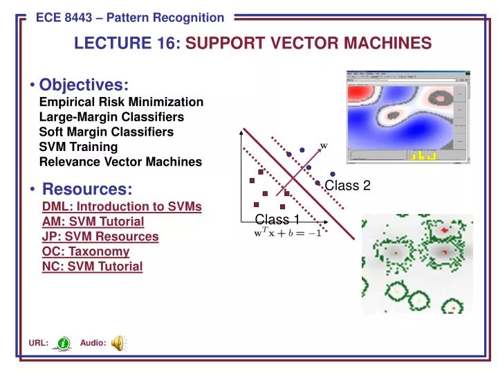
LECTURE 16: SUPPORT VECTOR MACHINES. Objectives: Empirical Risk Minimization Large-Margin Classifiers Soft Margin Classifiers SVM Training Relevance Vector Machines Resources: DML: Introduction to SVMs AM: SVM Tutorial JP: SVM Resources OC: Taxonomy NC: SVM Tutorial. Class 2. Class 1.

E N D
LECTURE 16: SUPPORT VECTOR MACHINES • Objectives:Empirical Risk MinimizationLarge-Margin ClassifiersSoft Margin ClassifiersSVM TrainingRelevance Vector Machines • Resources:DML: Introduction to SVMsAM: SVM TutorialJP: SVM ResourcesOC: TaxonomyNC: SVM Tutorial Class 2 Class 1 Audio: URL:
Generative Models • Thus far we have essentially considered techniques that perform classification indirectly by modeling the training data, optimizing the parameters of that model, and then performing classification by choosing the closest model. This approach is known as a generative model: by training models supervised learning assumes we know the form of the underlying density function, which is often not true in real applications. • Convergence in maximum likelihood does not guarantee optimal classification. • Gaussian MLE modeling tends tooverfit data. • Real data often not separable by hyperplanes. • Goal: balance representation and discrimination in a common framework (rather than alternating between the two).
Risk Minimization • The expected risk can be defined as: • Empirical risk is defined as: • These are related by the Vapnik-Chervonenkis (VC) dimension: where • is referred to as the VC confidence, where is a confidence measure in the range [0,1]. • The VC dimension, h, is a measure of the capacity of the learning machine. • The principle of structural risk minimization (SRM) involves finding the subset of functions that minimizes the bound on the actual risk. • Optimal hyperplane classifiers achieve zero empirical risk for linearly separable data. • A Support Vector Machine is an approach that gives the least upper bound on the risk.
Large-Margin Classification • Hyperplanes C0 - C2 achieve perfect classification(zero empirical risk): • C0 is optimal in terms of generalization. • The data points that define the boundaryare called support vectors. • A hyperplane can be defined by: • We will impose the constraints: • The data points that satisfy the equality arecalled support vectors. • Support vectors are found using a constrained optimization: • The final classifier is computed using the support vectors and the weights:
Class 2 Class 1 Soft-Margin Classification • In practice, the number of support vectors will grow unacceptably large for real problems with large amounts of data. • Also, the system will be very sensitive to mislabeled training data or outliers. • Solution: introduce “slack variables” or a soft margin: • This gives the system the ability toignore data points near the boundary,and effectively pushes the margintowards the centroid of the training data. • This is now a constrained optimizationwith an additional constraint: • The solution to this problem can still be found using Lagrange multipliers.
f( ) f( ) f( ) f( ) f( ) f( ) f( ) f( ) f( ) f( ) f( ) f( ) f( ) f( ) f( ) f( ) f( ) f( ) Nonlinear Decision Surfaces • Thus far we have only considered linear decision surfaces. How do we generalize this to a nonlinear surface? f(.) Feature space Input space • Our approach will be to transform the data to a higher dimensional space where the data can be separated by a linear surface. • Define a kernel function: • Examples of kernel functions include polynomial:
Kernel Functions Other popular kernels are a radial basis function (popular in neural networks): and a sigmoid function: • Our optimization does not change significantly: • The final classifier has a similar form: • Let’s work some examples.
SVM Limitations • Uses a binary (yes/no) decision rule • Generates a distance from the hyperplane, but this distance is often not a good measure of our “confidence” in the classification • Can produce a “probability” as a function of the distance (e.g. using sigmoid fits), but they are inadequate • Number of support vectors grows linearly with the size of the data set • Requires the estimation of trade-off parameter, C, via held-out sets Error Open-Loop Error Optimum Training Set Error Model Complexity
Build a fully specified probabilistic model – incorporate prior information/beliefs as well as a notion of confidence in predictions. MacKay posed a special form for regularization in neural networks – sparsity. Evidence maximization: evaluate candidate models based on their“evidence”, P(D|Hi). Evidence approximation: Likelihood of data given best fit parameter set: Penalty that measures how well our posterior modelfits our prior assumptions: We can use set the prior in favor of sparse,smooth models. Incorporates an automatic relevancedetermination (ARD) prior over each weight. P(w|D,Hi) D w P(w|Hi) w s w Evidence Maximization
Still a kernel-based learning machine: Incorporates an automatic relevance determination (ARD) prior over each weight (MacKay) A flat (non-informative) prior over a completes the Bayesian specification. The goal in training becomes finding: Estimation of the “sparsity” parameters is inherent in the optimization – no need for a held-out set. A closed-form solution to this maximization problem is not available. Rather, we iteratively reestimate . : Relevance Vector Machines
Summary • Support Vector Machines are one example of a kernel-based learning machine that is training in a discriminative fashion. • Integrates notions of risk minimization, large-margin and soft margin classification. • Two fundamental innovations: • maximize the margin between the classes using actual data points, • rotate the data into a higher-dimensional space in which the data is linearly separable. • Training can be computationally expensive but classification is very fast. • Note that SVMs are inherently non-probabilistic (e.g., non-Bayesian). • SVMs can be used to estimate posteriors by mapping the SVM output to a likelihood-like quantity using a nonlinear function (e.g., sigmoid). • SVMs are not inherently suited to an N-way classification problem. Typical approaches include a pairwise comparison or “one vs. world” approach.
Summary • Many alternate forms include Transductive SVMs, Sequential SVMs, Support Vector Regression, Relevance Vector Machines, and data-driven kernels. • Key lesson learned: a linear algorithm in the feature space is equivalent to a nonlinear algorithm in the input space. Standard linear algorithms can be generalized (e.g., kernel principal component analysis, kernel independent component analysis, kernel canonical correlation analysis, kernel k-means). • What we didn’t discuss: • How do you train SVMs? • Computational complexity? • How to deal with large amounts of data? • See Ganapathiraju for an excellent, easy to understand discourse on SVMs and Hamaker (Chapter 3) for a nice overview on RVMs. There are many other tutorials available online (see the links on the title slide) as well. • Other methods based on kernels – more to follow.