Download

1 / 19
190 likes | 351 Views
Estimating Surface Flows from HMI Magnetograms. GOAL : Consider techniques available to estimate flows from HMI vector magnetograms, to recommend which to employ in the HMI pipeline. Brian Welsch, SSL UC-Berkeley. Considerations. Accuracy of estimated flows

E N D
Estimating Surface Flows from HMI Magnetograms GOAL: Consider techniques available to estimate flows from HMI vector magnetograms, to recommend which to employ in the HMI pipeline. Brian Welsch, SSL UC-Berkeley
Considerations • Accuracy of estimated flows MEF; DAVE4VM; DAVE/FLCT; inductive correction 2. Data rate ~20 min. --- if inductivity matters, and if MDI is any guide 3. Processing rate DAVE4VM, DAVE, FLCT are fast, and parallelizable • Noise handling DAVE4VM, DAVE, FLCT handle noise well, but other approaches are possible.
Recently, we conducted quantitative tests of accuracy using several available methods. - We created “synthetic magnetograms” from ANMHD simulations of an emerging flux rope.- In these data, both v & B are known exactly.
Via several methods, we estimated v from N= 7 pairs of magnetograms, with increasing Δt’s. • We verified that the ANMHD data were consistent with ∂tBn= ∙(vnBhor- vhorBn). • Here, I show representative results from just a few of the methods tested: • Fourier LCT (FLCT, Welsch et al. 2004) • Inductive LCT (ILCT, Welsch et al. 2004) • Minimum Energy Fit (MEF, Longcope 2004) • Differential Affine Velocity Estimator (DAVE, Schuck 2006) … 5. DAVE4VM (Schuck 2008) --- DAVE for vector m’grams
We verified the methods’ inductivity, i.e., that they satisfy ∂tBn = ∙ (vnBhor– vhorBn). ILCT FLCT DAVE MEF
Estimated v’s are highly correlated with ANMHD’s v.. FLCT ILCT MEF DAVE
Not surprisingly, the methods’ performance worsened as the time between magnetograms increased. % vector errors (direction & magnitude) were at least 50% (!!!). % speed errors (magnitude) were smaller, but biases were seen.
Schuck has developed DAVE4VM, a new version of DAVE meant for vector magnetograms. A manuscript is posted on arXiv.org, at http://arxiv.org/abs/0803.3472 Flows from DAVE4VM are as accurate as the best of the methods tested by Welsch et al. (2007), though its Poynting flux estimates are slightly worse than MEF’s.
Considerations • Accuracy of estimated flows MEF; DAVE4VM; DAVE/FLCT; inductive correction 2. Data rate ~20 min. --- if inductivity matters, and if MDI is any guide 3. Processing rate DAVE4VM, DAVE, FLCT are fast, and parallelizable • Noise handling DAVE4VM, DAVE, FLCT handle noise well, but other approaches are possible.
Pixel size and timescales of rotation & magnetic evolution affect optimal data rate. • Target HMI resolution is 1” (Schou 2005*), or ~ 725 km at the Sun (cf., pixel size = 0.5”) • Here, I assume rebinning, so Δx ≈ 1” Pixels. (I’ll try to use capital P for rebinned Pix.) • Typical flows are vtyp~ 1 km/ sec. Δt ≈ 12 min. (Rotation rate is 2 km/ sec. Δt ≈ 6 min. But rotation can be systematically removed.) * J. Schou, “Instrument Performance and Requirements,“ HMI Team Mtg. ‘05
This data rate is slow enough that ΔBn(F) from flows exceeds ΔBn(N) from noise. Since ΔBn(F)= Δtminhor·(vn Bhor - vhor Bn) ΔBn(F) ~ Δtmin(Btyp vtyp)/ Δx > ΔBn(N) Δtmin > ΔBn(N)Δx / (Btyp vtyp) If Bz meets HMI noise target (Schou 2005), then σB ~10 G, soΔBn(N)~ sqrt(2) σB ~ 14 G. With Btyp~100 G, Δtmin > 100 sec. ~ 1.6 min. Linear in ΔBz(N)
“Inductivity” might be an objective measure of consistency when flows are not known. “Inductivity” is how well hor·(vn Bhor - vhor Bn) matches ΔBn/Δt Rieutord et al. (2001) argue that (1) spatial windowing during tracking, and (2) large Δt effectively average smaller-scale velocities. These can undermine the inductivity as a test of consistency.
Inductivity is affected both by averaging Binitial and Bfinal to reduce noise, and data’s Δt. Avg. of five 1-min. cadence magnetograms prior to computing ΔB(right) improves inductivity compared to using unaveraged ΔB (left).
Inductivity is affected both by averaging Binitial and Bfinal to reduce noise, and data’s Δt. 12 min. 18 min. 36 min. 54 min.
Considerations • Accuracy of estimated flows MEF; DAVE4VM; DAVE/FLCT; inductive correction 2. Data rate ~20 min. --- if inductivity matters, and if MDI is any guide 3. Processing rate DAVE4VM, DAVE, FLCT are fast, and parallelizable • Noise handling DAVE4VM, DAVE, FLCT handle noise well, but other approaches are possible.
*Both DAVE and FLCT are trivially parallelizable. Matching HMI’s 10-minute vector magnetogram cadence is feasible, with DAVE (or FLCT). • HMI has Npix ~ 3 x 10⁶ Pixels within 60o of disk center. • - 2x rebin of 40962 20482 Pix • - w/in ~60o (0.866)2 x 20482 Pix ~ 3 MPix • Only tracking pixels if |Bn| > |B|thresh , for |B|thr=20 G, • ~ 25% of Npix at solar max. for MDI 750 kPix • ~ 5% of Npix at solar min. for MDI 150 kPix • DAVE tracks ~ 4 kPix/sec** in IDL (!), with one CPU* • - FLCT tracks ~ 1kPix/sec in C, with one CPU • - t ~ (1 sec/1 kPix) x (750 kPix) ~ 750 sec ~ 12 min! • - at solar min., w/ |B|thresh = 100G (~1% of Npix), t ~ 30 sec. ** DAVE4VM will be slower --- probably by a factor of 3.
Considerations • Accuracy of estimated flows MEF; DAVE4VM; DAVE/FLCT; inductive correction 2. Data rate ~20 min. --- if inductivity matters, and if MDI is any guide 3. Processing rate DAVE4VM, DAVE, FLCT are fast, and parallelizable • Noise handling DAVE4VM, DAVE, FLCT handle noise well, but other approaches are possible.
The induction equation can be solved to roundoff error, but data noise can make this undesirable. • DAVE, DAVE4VM, and LCT codes solve for window-averaged flows, so average over noise --- a good thing! • DAVE & DAVE4VM use least-squares fitting to determine flows --- also good for dealing with noise. • ILCT and MEF solve the induction equation exactly, which tends to produce spiky flows. • Regularization to enforce smoothness, or the Kalman filter might enable combining “local” tracking results with “global” exact methods. This is ongoing research!
Considerations • Accuracy of estimated flows MEF; DAVE4VM; DAVE/FLCT; inductive correction 2. Data rate ~20 min. --- if inductivity matters, and if MDI is any guide 3. Processing rate DAVE4VM, DAVE, FLCT are fast, and parallelizable • Noise handling We expect DAVE4VM, DAVE, FLCT to handle noise well (but still need to test this), & other approaches might work.