Download
1 / 39
390 likes | 541 Views
Introduction to Using Radio Telescopes. Frank Ghigo, NRAO-Green Bank. The Fifth NAIC-NRAO School on Single-Dish Radio Astronomy July 2009. Introduction to Using Radio Telescopes. Frank Ghigo, NRAO-Green Bank. The Fifth NAIC-NRAO School on Single-Dish Radio Astronomy July 2009.

E N D
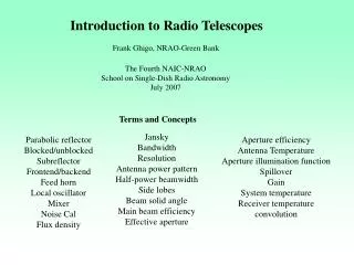
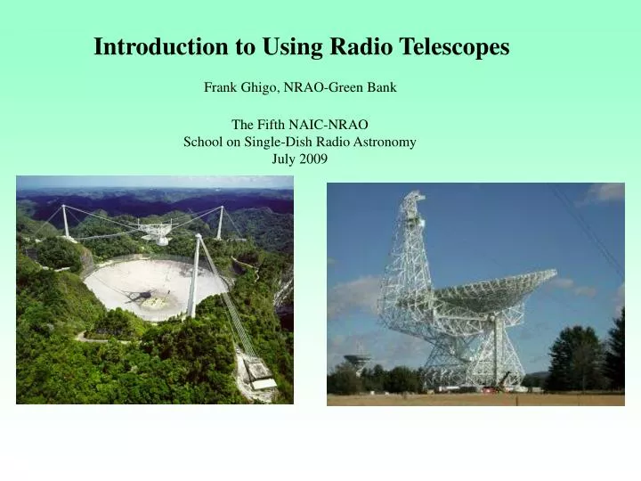
Introduction to Using Radio Telescopes Frank Ghigo, NRAO-Green Bank The Fifth NAIC-NRAO School on Single-Dish Radio Astronomy July 2009
Introduction to Using Radio Telescopes Frank Ghigo, NRAO-Green Bank The Fifth NAIC-NRAO School on Single-Dish Radio Astronomy July 2009 Terms and Concepts Jansky Bandwidth Resolution Antenna power pattern Half-power beamwidth Side lobes Beam solid angle Main beam efficiency Effective aperture Parabolic reflector Blocked/unblocked Subreflector Frontend/backend Feed horn Local oscillator Mixer Noise Cal Flux density Aperture efficiency Antenna Temperature Aperture illumination function Spillover Gain System temperature Receiver temperature convolution
Pioneers of Radio Astronomy Grote Reber 1938 Karl Jansky 1932
Unblocked Aperture • 100 x 110 m section of a parent parabola 208 m in diameter • Cantilevered feed arm is at focus of the parent parabola
Basic Radio Telescope Verschuur, 1985. Slide set produced by the Astronomical Society of the Pacific, slide #1.
Intrinsic Power P (Watts)Distance R (meters)Aperture A (sq.m.) Flux = Power/Area Flux Density (S) = Power/Area/bandwidth Bandwidth () A “Jansky” is a unit of flux density
Antenna Beam Pattern (power pattern) Beam solid angle (steradians) Main Beam Solid angle Pn = normalized power pattern Kraus, 1966. Fig.6-1, p. 153.
Some definitions and relations Directivity or Directive Gain Main beam efficiency, M Antenna theorem Aperture efficiency, ap Effective aperture, Ae Geometric aperture, Ag
Directive gains for GBT, Arecibo For = 21cm, e=0.7 (Gregorian)
Aperture feed pattern, or illumination pattern. Kraus, 1966. Fig.1-6, p. 14.
Aperture Illumination FunctionandBeam Patternare Fourier transforms of each other A gaussian aperture illumination gives a gaussian beam: Kraus, 1966. Fig.6-9, p. 168.
Surface efficiency -- Ruze formula = rms surface error Effect of surface efficiency John Ruze of MIT -- Proc. IEEE vol 54, no. 4, p.633, April 1966.
Detected power (W, watts) from a resistor R at temperature T (kelvin) over bandwidth (Hz) Power WA detected in a radio telescope Due to a source of flux density S power as equivalent temperature. Antenna Temperature TA Effective Aperture Ae
Gain (or sensitivity) (K/Jy) GBT: Arecibo: (Gregorian:) Correct for atmospheric absorption:
System Temperature = total noise power detected, a result of many contributions Thermal noise T = minimum detectable signal For GBT spectroscopy
Convolution relationfor observed brightness distribution Thompson, Moran, Swenson, 2001. Fig 2.5, p. 58.
Smoothing by the beam Kraus, 1966. Fig. 3-6. p. 70; Fig. 3-5, p. 69.
Physical temperature vs antenna temperature For an extended object with source solid angle s, And physical temperature Ts, then for for In general :
Calibration: Scan of Cass A with the 40-Foot. peak baseline Tant = Tcal * (peak-baseline)/(cal – baseline) (Tcal is known)
More Calibration : GBT Convert counts to T
GBT active surface system • Surface has 2004 panels • average panel rms: 68 m • 2209 precision actuators • Designed to operate in: • open loop from look-up table
Surface Panel Actuators One of 2209 actuators. • Actuators are located under each set of surface panel corners • Actuator Control Room • 26,508 control and supply wires terminated in this room
Surface efficiency -- Ruze formula = rms surface error Effect of surface efficiency John Ruze of MIT -- Proc. IEEE vol 54, no. 4, p.633, April 1966.
Improving the surface for High-Frequency Performance: • Surface • Mechanical adjustments • Photogrammetry • FEM (finite element model) • OOF (“out of focus” holography) model - global • AutoOOF - correct thermal errors short term • “Traditional” holography
OOF: out of focus “holography” Zernike polynomials