Download
1 / 58
580 likes | 582 Views
Understand the challenges of achieving global time and state in distributed systems and learn about clock synchronization algorithms and their accuracy.

E N D
Distributed Computing Concepts - Global Time and State in Distributed Systems Prof. Nalini Venkatasubramanian Distributed Systems Middleware - Lecture 2
Global Time & Global States of Distributed Systems • Asynchronous distributed systems consist of several processes without common memory which communicate (solely) via messageswith unpredictable transmission delays • Global time & global state are hard to realize in distributed systems • Rate of event occurrence is very high • Event execution times are very small • We can only approximate the global view • Simulatesynchronous distributed system on a given asynchronous systems • Simulate a global time – Clocks (Physical and Logical) • Simulate a global state – Global Snapshots
Simulate Synchronous Distributed Systems • Synchronizers [Awerbuch 85] • Simulate clock pulses in such a way that a message is only generated at a clock pulse and will be received before the next pulse • Drawback • Very high message overhead
The Concept of Time in Distributed Systems • A standard time is a set of instants with a temporal precedence order < satisfying certain conditions [Van Benthem 83]: • Irreflexivity • Transitivity • Linearity • Eternity (xy: x<y) • Density (x,y: x<y z: x<z<y) • Transitivity and Irreflexivity imply asymmetry • A linearly ordered structure of time is not always adequate for distributed systems • Captures dependence, not independence of distributed activities • Time as a partial order • A partially ordered system of vectors forming a lattice structure is a natural representation of time in a distributed system
Global time in distributed systems • An accurate notion of global time is difficult to achieve in distributed systems. • Uniform notion of time is necessary for correct operation of many applications (mission critical distributed control, online games/entertainment, financial apps, smart environments etc.) • Clocks in a distributed system drift • Relative to each other • Relative to a real world clock • Determination of this real world clock itself may be an issue • Clock synchronization is needed to simulate global time • Physical Clocks vs. Logical clocks • Physical clocks are logical clocks that must not deviate from the real-time by more than a certain amount. We often derive causality of events from loosely synchronized clocks
Physical Clocks • How do we measure real time? • 17th century - Mechanical clocks based on astronomical measurements • Solar Day - Transit of the sun • Solar Seconds - Solar Day/(3600*24) • Problem (1940) - Rotation of the earth varies (gets slower) • Mean solar second - average over many days
Atomic Clocks • 1948 • Counting transitions of a crystal (Cesium 133, quartz) used as atomic clock • crystal oscillates at well known frequency • TAI - International Atomic Time • 9192631779 transitions = 1 mean solar second in 1948 • UTC (Universal Coordinated Time) • From time to time, we skip a solar second to stay in phase with the sun (30+ times since 1958) • UTC is broadcast by several sources (satellites…)
How Clocks Work in Computers Oscillation at a well-defined frequency Quartz crystal Holding register Each crystal oscillation decrements the counter by 1 When counter gets 0, its value reloaded from the holding register Counter When counter is 0, an interrupt is generated, which is call a clock tick CPU At each clock tick, an interrupt service procedure add 1 to time stored in memory Memory From Distributed Systems (cs.nju.edu.cn/distribute-systems/lecture-notes/
Accuracy of Computer Clocks • Modern timer chips have a relative error of 1/100,000 - 0.86 seconds a day • To maintain synchronized clocks • Can use UTC source (time server) to obtain current notion of time • Use solutions without UTC.
Cristian’s (Time Server) Algorithm • Uses a time server to synchronize clocks • Time server keeps the reference time (say UTC) • A client asks the time server for time, the server responds with its current time, and the client uses the received value to set its clock • But network round-trip time introduces errors… • Let RTT = response-received-time – request-sent-time (measurable at client), • If we know (a) min = minimum client-server one-way transmission time and (b) that the server timestamped the message at the last possible instant before sending it back • Then, the actual time could be between [T+min,T+RTT— min]
Cristian’s Algorithm • Client sets its clock to halfway between T+minandT+RTT— min i.e., at T+RTT/2 Expected (i.e., average) skew in client clock time = (RTT/2 – min) • Can increase clock value, should never decrease it. • Can adjust speed of clock too (either up or down is ok) • Multiple requests to increase accuracy • For unusually long RTTs, repeat the time request • For non-uniform RTTs • Drop values beyond threshold; Use averages (or weighted average)
Berkeley UNIX algorithm • One daemon without UTC • Periodically, this daemon polls and asks all the machines for their time • The machines respond. • The daemon computes an average time and then broadcasts this average time.
Decentralized Averaging Algorithm • Each machine has a daemon without UTC • Periodically, at fixed agreed-upon times, each machine broadcasts its local time. • Each of them calculates the average time by averaging all the received local times.
DCE Distributed Time Service • Software service that provides precise, fault-tolerant clock synchronization for systems in local area networks (LANs) and wide area networks (WANs). • determine duration, perform event sequencing and scheduling. • Each machine is either a time server or a clerk • software components on a group of cooperating systems; • client obtains time from DTSentity • DTS entities • DTSserver • DTSclerk that obtain time from DTS servers on other hosts
Clock Synchronization in DCE • DCE’s time model is actually in an interval • I.e. time in DCE is actually an interval • Comparing 2 times may yield 3 answers • t1 < t2, t2 < t1, not determined • Periodically a clerk obtains time-intervals from several servers ,e.g. all the time servers on its LAN • Based on their answers, it computes a new time and gradually converges to it. • Compute the intersection where the intervals overlap. Clerks then adjust the system clocks of their client systems to the midpoint of the computed intersection. • When clerks receive a time interval that does not intersect with the majority, the clerks declare the non-intersecting value to be faulty. • Clerks ignore faulty values when computing new times, thereby ensuring that defective server clocks do not affect clients.
Network Time Protocol (NTP) • Most widely used physical clock synchronization protocol on the Internet (http://www.ntp.org) • Currently used: NTP V3 and V4 • 10-20 million NTP servers and clients in the Internet • Claimed Accuracy (Varies) • milliseconds on WANs, submilliseconds on LANs, submicroseconds using a precision timesource • Nanosecond NTP in progress
NTP Design • Hierarchical tree of time servers. • The primary server at the root synchronizes with the UTC. • The next level contains secondary servers, which act as a backup to the primary server. • At the lowest level is the synchronization subnet which has the clients.
Causal Relations • Distributed application results in a set of distributed events • Induces a partial order causal precedence relation • Knowledge of this causal precedence relation is useful in reasoning about and analyzing the properties of distributed computations • Liveness and fairness in mutual exclusion • Consistency in replicated databases • Distributed debugging, checkpointing
Logical Clocks • Used to determine causality in distributed systems • Time is represented by non-negative integers • Event structures represent distributed computation (in an abstract way) • A process can be viewed as consisting of a sequence of events, where an event is an atomic transition of the local state which happens in no time • Process Actions can be modeled using the 3 types of events • Send Message • Receive Message • Internal (change of state)
Logical Clocks • A logical Clock C is some abstract mechanism which assigns to any event eE the value C(e) of some time domain T such that certain conditions are met • C:ET :: T is a partially ordered set : e<e’C(e)<C(e’) holds • Consequences of the clock condition [Morgan 85]: • Events occurring at a particular process are totally ordered by their local sequence of occurrence • If an event e occurs before event e’ at some single process, then event e is assigned a logical time earlier than the logical time assigned to event e’ • For any message sent from one process to another, the logical time of the send event is always earlier than the logical time of the receive event • Each receive event has a corresponding send event • Future can not influence the past (causality relation)
Event Ordering • Lamport defined the “happens before” (=>) relation • If a and b are events in the same process, and a occurs before b, then a => b. • If a is the event of a message being sent by one process and b is the event of the message being received by another process, then a => b. • If X =>Y and Y=>Z then X => Z. If a => b then time (a) => time (b)
global time e11 e13 e12 e14 P1 Program order: e13 < e14 Send-Receive: e23 < e12 Transitivity: e21 < e32 e21 e22 e23 P2 e31 e32 P3 Event Ordering- the example Processor Order: e precedes e’ in the same process Send-Receive: e is a send and e’ is the corresponding receive Transitivity: exists e’’ s.t. e < e’’ and e’’< e’ Example:
Causal Ordering • “Happens Before” also called causal ordering • Possible to draw a causality relation between 2 events if • They happen in the same process • There is a chain of messages between them • “Happens Before” notion is not straightforward in distributed systems • No guarantees of synchronized clocks • Communication latency
Implementation of Logical Clocks • Requires • Data structures local to every process to represent logical time and • a protocol to update the data structures to ensure the consistency condition. • Each process Pi maintains data structures that allow it the following two capabilities: • A local logical clock, denoted by LC_i , that helps process Pi measure its own progress. • A logical global clock, denoted by GCi , that is a representation of process Pi ’s local view of the logical global time. Typically, lci is a part of gci • The protocol ensures that a process’s logical clock, and thus its view of the global time, is managed consistently. • The protocol consists of the following two rules: • R1: This rule governs how the local logical clock is updated by a process when it executes an event. • R2: This rule governs how a process updates its global logical clock to update its view of the global time and global progress.
Types of Logical Clocks • Systems of logical clocks differ in their representation of logical time and also in the protocol to update the logical clocks. • 3 kinds of logical clocks • Scalar • Vector • Matrix
Scalar Logical Clocks - Lamport • Proposed by Lamport in 1978 as an attempt to totally order events in a distributed system. • Time domain is the set of non-negative integers. • The logical local clock of a process pi and its local view of the global time are squashed into one integer variable Ci . • Monotonically increasing counter • No relation with real clock • Each process keeps its own logical clock used to timestamp events
Consistency with Scalar Clocks • To guarantee the clock condition, local clocks must obey a simple protocol: • When executing an internal event or a send event at process Pi the clock Ci ticks • Ci += d (d>0) • When Pi sends a message m, it piggybacks a logical timestamp t which equals the time of the send event • When executing a receive event at Pi where a message with timestamp t is received, the clock is advanced • Ci = max(Ci,t)+d (d>0) • Results in a partial ordering of events.
Total Ordering • Extending partial order to total order • Global timestamps: • (Ta, Pa) where Ta is the local timestamp and Pa is the process id. • (Ta,Pa) < (Tb,Pb) iff • (Ta < Tb) or ( (Ta = Tb) and (Pa < Pb)) • Total order is consistent with partial order. time Proc_id
Independence Two events e,e’ are mutually independent (i.e. e||e’) if ~(e<e’)~(e’<e) Two events are independent if they have the same timestamp Events which are causally independent may get the same or different timestamps By looking at the timestamps of events it is not possible to assert that some event could not influence some other event If C(e)<C(e’) then ~(e’<e)however, it is not possible to decide whether e<e’ or e||e’ C is an order homomorphism which preserves < but it does not preserves negations (i.e. obliterates a lot of structure by mapping E into a linear order)
Problems with Total Ordering • A linearly ordered structure of time is not always adequate for distributed systems • captures dependence of events • loses independence of events - artificially enforces an ordering for events that need not be ordered – loses information • Mapping partial ordered events onto a linearly ordered set of integers is losinginformation • Events which may happen simultaneously may get different timestamps as if they happen in some definite order. • A partially ordered system of vectors forming a lattice structure is a natural representation of time in a distributed system
Vector Times • The system of vector clocks was developed independently by Fidge, Mattern and Schmuck. • To construct a mechanism by which each process gets an optimal approximation of global time • In the system of vector clocks, the time domain is represented by a set of n-dimensional non-negative integer vectors. • Each process has a clock Ci consisting of a vector of length n, where n is the total number of processes vt[1..n], where vt[j ] is the local logical clock of Pj and describes the logical time progress at process Pj . • A process Pi ticks by incrementing its own component of its clock • Ci[i] += 1 • The timestamp C(e) of an event e is the clock value after ticking • Each message gets a piggybacked timestamp consisting of the vector of the local clock • The process gets some knowledge about the other process’ time approximation • Ci=sup(Ci,t):: sup(u,v)=w : w[i]=max(u[i],v[i]), i
Vector Clocks example • An Example of vector clocks Figure 3.2: Evolution of vector time. From A. Kshemkalyani and M. Singhal (Distributed Computing)
Vector Times (cont) • Because of the transitive nature of the scheme, a process may receive time updates about clocks in non-neighboring process • Since process Pi can advance the ith component of global time, it always has the most accurate knowledge of its local time • At any instant of real time i,j: Ci[i] Cj[i] • For two time vectors u,v • uv iff i: u[i]v[i] • u<v iff uv uv • u||v iff ~(u<v) ~(v<u) :: || is not transitive
Structure of the Vector Time • For any n>0, (Nn,) is a lattice • The set of possible time vectors of an event set E is a sublattice of (Nn,) • For an event set E, the lattice of consistent cuts and the lattice of possible time vectors are isomorphic • e,e’E:e<e’ iff C(e)<C(e’) e||e’ iff iff C(e)||C(e’) • In order to determine if two events e,e’ are causally related or not, just take their timestamps C(e) and C(e’) • if C(e)<C(e’) C(e’)<C(e), then the events are causally related • Otherwise, they are causally independent
Matrix Time • Vector time contains information about latest direct dependencies • What does Pi know about Pk • Also contains info about latest direct dependencies of those dependencies • What does Pi know about what Pk knows about Pj • Message and computation overheads are high • Powerful and useful for applications like distributed garbage collection
Time Manager Operations • Logical Clocks • C.adjust(L,T) • adjust the local time displayed by clock C to T (can be gradually, immediate, per clock sync period) • C.read • returns the current value of clock C • Timers • TP.set(T) - reset the timer to timeout in T units • Messages • receive(m,l); broadcast(m); forward(m,l)
Simulate A Global State • The notions of global time and global state are closely related • A process can (without freezing the whole computation) compute the bestpossibleapproximation of a global state [Chandy & Lamport 85] • A global state that could have occurred • No process in the system can decide whether the state did really occur • Guarantee stable properties (i.e. once they become true, they remain true)
Event Diagram Time e11 e12 e13 P1 e21 e22 e23 e24 e25 P2 e32 e33 e34 P3 e31
Equivalent Event Diagram Time e11 e12 e13 P1 e21 e22 e23 e24 e25 P2 e32 e33 e34 P3 e31
Rubber Band Transformation Time e11 e12 P1 e21 e22 P2 P3 e31 P4 e41 e42 cut
Poset Diagram e34 e13 e33 e12 e25 e32 e24 e23 e22 e11 e21 e31
Poset Diagram e22 e12 e21 e42 e31 Past e41 e21
Consistent Cuts • A cut (or time slice) is a zigzag line cutting a time diagram into 2 parts (past and future) • E is augmented with a cut event ci for each process Pi:E’ =E {ci,…,cn} • A cut C of an event set E is a finite subset CE: eC e’<le e’C • A cut C1 is later than C2 if C1C2 • A consistent cut C of an event set E is a finite subset CE : eC e’<e e’ C • i.e. a cut is consistent if every message received was previously sent (but not necessarily vice versa!)
Cuts (Summary) Instant of local observation Time P1 5 8 3 initial value P2 5 2 3 7 4 1 P3 5 4 0 ideal (vertical) cut (15) consistent cut (15) inconsistent cut (19) not attainable equivalent to a vertical cut (rubber band transformation) can’t be made vertical (message from the future) “Rubber band transformation” changes metric, but keeps topology
Consistent Cuts • Some Theorems • For a consistent cut consisting of cut events ci,…,cn, no pair of cut events is causally related. i.e ci,cj ~(ci< cj) ~(cj< ci) • For any time diagram with a consistent cut consisting of cut events ci,…,cn, there is an equivalent time diagram where ci,…,cn occur simultaneously. i.e. where the cut line forms a straight vertical line • All cut events of a consistent cut can occur simultaneously
Global States of Consistent Cuts • The global state of a distributed system is a collection of the local states of the processes and the channels. • A global state computed along a consistent cut is correct • The global state of a consistent cut comprises the local state of each process at the time the cut event happens and the set of all messages sent but not yet received • The snapshot problem consists in designing an efficient protocol which yields only consistent cuts and to collect the local state information • Messages crossing the cut must be captured • Chandy & Lamport presented an algorithm assuming that message transmission is FIFO
System Model for Global Snapshots • The system consists of a collection of n processes p1, p2, ..., pn that are connected by channels. • There are no globally shared memory and physical global clock and processes communicate by passing messages through communication channels. • Cij denotes the channel from process pi to process pj and its state is denoted by SCij . • The actions performed by a process are modeled as three types of events: • Internal events,the message send event and the message receive event. • For a message mij that is sent by process pi to process pj , let send(mij ) and rec(mij ) denote its send and receive events.