Chris Brien 1 & Clarice Demétrio 2

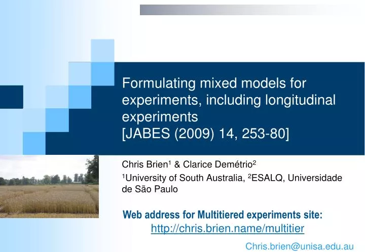
1. Formulating mixed models for experiments, including longitudinal experiments [JABES (2009) 14, 253-80] Chris Brien1 & Clarice Demétrio2 1University of South Australia, 2ESALQ, Universidade de São Paulo Web address for Multitiered experiments site: http://chris.brien.name/multitier Chris.brien@unisa.edu.au

2. Outline • Three-stage method • Randomization diagrams & tiers • Symbolic mixed model notation • A longitudinal Randomized Complete Block Design (RCBD) • A three-phase example • Concluding comments

3. 1. Three-stage method (motivated by Piepho et al., 2004);extension of Brien and Bailey, 2006, section 7) I. Intratier Random and Intratier Fixed models: Essentially models equivalent to a randomization model. Homogeneous Random and Fixed models:Terms added to intratier models and others shifted between intratier random and intratier fixed models. II. • Up to here have ANOVA models General Random and General Fixed models:Perhaps reparameterize terms in homogeneous models, particularly if a longitudinal experiment, and omit aliased terms from random model. III. • May yield a model of convenience, not full mixed model. Fundamental is experiment description starts with tiers

4. randomized unrandomized bBlocks tRunsin B bt units tTreatments t treatments a) Randomization diagrams & tiers (Brien, 1983; Brien & Bailey, 2006) RCBD – two-tiered • A panel for a set of objects shows: • a list of the factors in a tier; their numbers of levels; their nesting relationships. • So a tier is just a set of factors: • {Treatments} or {Blocks, Runs} • But, not just any old set: a) factors that belong to an object and b) a set of factors with the same status in the randomization. • Textbook experiments are two-tiered, but in practice some experiments are multitiered. • A crucial feature is that diagram automatically shows EU and restrictions on randomization.

5. Why have tiers? • Would not be need if all experiments were two-tiered, as only two sets of factors needed. • Various names used for the two sets of factors: • block or unit or unrandomized factors; • treatment or randomized factors. • These would be sufficient. • However, some experiments have three or more sets of factors. • Instead of naming each set, use tiers as a general term for these sets. • i.e. for sets of factors based on the randomization. • Will present an example with 4 tiers

6. Single-set description e.g. Searle, Casella & McCulloch (1992); Littel et al. (2006). • Single set of factors that uniquely indexes observations: • {Blocks, Treatments} • A subset of the factors from the randomization description. • {Treatments} and {Blocks, Runs} • What are the EUs in this approach? • A set of units that are indexed by Blocks x Treatments combinations. • Of course, Blocks x Treats are not the actual EUs, as Treats not randomized to those combinations. • They act as a proxy for the unnamed units. • Tier-based (and so multi-set) description has a specific factor for the Eus: • identity of EUs not obscured; • runs indexed by Blocks-Runs combinations to which Treats are randomized.

7. b) Symbolic mixed model notation Generalized factor = term in mixed model: AB is the ab-level factor formed from the combinations of A with a levels and B with b levels. Symbolic mixed model Fixed terms | random terms Factor relationships used to get generalized factors from each panel A*B factors A and B are crossed; A/B factor B is nested within A. Example: A*B | Blocks/Runs • A + B + AB | Blocks + BlocksRuns

8. More general mixed models • Modify randomization model to allow for intertier interactions and other forms of models • Use functions on generalized factors (borrowed from ASReml-R). For random terms: uc(.) some, possibly structured, form of unequal correlation between levels of the generalized factor. ar1(.), corb(.), us(.) are examples of specific structures. h added to correlation function allows for heterogeneous variances: uch, ar1h, corbh, ush. For fixed models terms: td(.) systematic trend across levels of the generalized factor. lin(.), pol(.), spl(.) are examples of specific trend functions.

9. 2) A longitudinal RCBD (Piepho et al., 2004, Example 1) Lay 4 Lay 3 Lay 2 Lay 1 Block 1 Plot 3 Plot 2 Plot 1 Block 2 Plot 1 Plot 3 Plot 2 4 Blocks 3 Plotsin B 4 Lay Block 3 Plot 2 Plot 1 Plot 3 3 Tillage Plot 3 Plot 2 Plot 1 Block 4 3 treatments 48 layer-plots A field experiment comparing 3 different tillage methods Laid out according to an RCBD with 4 blocks. On each plot one water collector is installed in each of 4 layers and the amount of nitrogen leaching measured.

10. Specific longitudinal terminology Lay 4 Lay 3 Lay 2 Lay 1 Block 1 Plot 3 Plot 2 Plot 1 Block 2 Plot 1 Plot 3 Plot 2 Block 3 Plot 2 Plot 1 Plot 3 Plot 3 Plot 2 Plot 1 Block 4 4 Blocks 3 Plotsin B 4 Lay 3 Tillage 3 treatments 48 layer-plots • Longitudinal factors: those a) to which no factors are randomized and b) that index successive observations of some entity. • Lay • A subject term for a longitudinal factor is a generalized factor whose levels are entities on which the successive observations are taken. • BlocksPlots (1,1; 1,2; 1,3; 2,1; and so on)

11. A longitudinal RCBD— Intratier random and intratier fixed models 4 Blocks 3 Plotsin B 4 Lay 3 Tillage 3 treatments 48 layer-plots I. • Intratier Random and Intratier Fixed models: • The unrandomized tier is {Block, Plot, Lay}; • The randomized tier is {Tillage}. • The only longitudinal factor is Lay. Intratier Random: (Block / Plot) * Lay = Block + Lay + BlockLay + BlockPlot + BlockPlotLay ; IntratierFixed: Tillage. • Have all possible terms given the randomization.

12. A longitudinal RCBD — Homogeneous random and fixed models I. Intratier Random: (Block / Plot) * Lay = Block + Lay + BlockLay + BlockPlot + BlockPlotLay ; IntratierFixed: Tillage. II. Homogeneous Random and Fixed models:Terms added to intratier models and others shifted from intratier random to intratier fixed models and vice versa. • Take the fixed factors to be Block, Tillage and Lay and the random factor to be Plot. • Terms involving just Block and Lay that are in the Intratier Random model are shifted to the fixed model. • Lay#Tillage is of interest so that the fixed model should include TillageLay. Homogeneous Random: BlockPlot + BlockPlotLay= (BlockPlot) / Lay Fixed: Block + Lay + BlockLay + Tillage + TillageLay= (Block + Tillage) * Lay

13. A longitudinal RCBD — General random and general fixed models II. Homogeneous Random: BlockPlot + BlockPlotLay= (BlockPlot) / Lay Fixed: Block + Lay + BlockLay + Tillage + TillageLay= (Block + Tillage) * Lay III. General Random and General Fixed models:Reparameterize terms in homogeneous models and omit aliased terms from random model. • For longitudinal experiments, form longitudinal error terms: (subject term)gf(longitudinal factors): • Allow unequal correlation (uc) between longitudinal factor levels; • Use gf on longitudinal factors: list unique factors separated by ‘’; allows arbitrary uc between these factors. • The subject term for Lay is BlockPlot; • Expected that there will be unequal correlation between observations with different levels of Lay and same levels of BlockPlot; • No aliased random terms. • General random: (BlockPlot) / uc(gf(Lay)) (BlockPlot) / uc(Lay) • Trends for Lay are of interest, but not for the qualitative factor Tillage nor for Block. Mixed model: (Block + Tilllage) * td(Lay) | (BlockPlot) / uc(Lay) General fixed: (Block + Tilllage) * td(Lay)

14. 3) A three-phase example (Pereira, 1969) 6 Times 2 Kinds 2 Ages 3 Lots in K, A 4 Batches in K, A, L 6 times 6 Samples in C 48 Cookings 6 Positions in R 48 Runs • Experiment to investigate differences between pulps produced from different Eucalypt trees. • Chip phase: • 3 lots of 5 trees from each of 4 areas were processed into wood chips. • Each area differed in i) kinds of trees (2 species) and ii) age (5 and 7 years). • For each of 12 lots, chips from 5 trees were combined and 4 batches selected. • Pulp phase: • Batches were cooked to produce pulp & 6 samples obtained from each cooking. • Measurement phase: • Each batch processed in one of 48 Runs of a laboratory refiner with its 6 samples randomly placed on 6 positions in a pan in the refiner. • For each run, 6 times of refinement (30, 60, 90, 120, 150 and 180 minutes) were randomized to the 6 positions in the pan. • After allotted time, a sample taken from a pan and its degree of refinement measured. 48 batches 288 samples 288 positions

15. Profile plot of data Shows: a) curvature in the trend over time; b) some trend variability; c) variance heterogeneity, in particular between the Ages which was included in fitted model [see Brien & Demétrio (2009) for details].

16. Predicted degree of refinement Same Age (differ in slope) Different Age (differ in intercept and curvature)

17. 5) Concluding comments • Formulate a randomization-based mixed model: • to ensure that all terms appropriate, given the randomization, are included; • and makes explicit where model deviates from a randomization model. • Based on dividing the factors in an experiment into tiers. • To obtain fit, a model of convenience is often used: • When aliased random sources, terms for all but one are omitted to obtain fit; • But re-included in fitted model if retained term is in fitted model. • All 11 examples from Piepho et al. (2004) are in Brien and Demétrio (2009), including: • An experiment with systematically applied treatments and another with crop rotations, both of which are not longitudinal.

18. References Brien, C.J., and Bailey, R.A. (2006) Multiple randomizations (with discussion). J. Roy. Statist. Soc., Ser. B, 68, 571–609. Brien, C.J. and Demétrio, C.G.B. (2009) Formulating mixed models for experiments, including longitudinal experiments. J. Agr. Biol. Env. Stat., 14, 253-80. Butler, D., Cullis, B.R., Gilmour, A.R. and Gogel, B.J. (2009) Analysis of mixed models for S language environments: ASReml-R reference manual. DPI Publications, Brisbane. Littel, R., Milliken, G., Stroup, W., Wolfinger, R. and Schabenberger, O. (2006) SAS for Mixed Models. 2nd edn. SAS Press, Cary. Pereira, R.A.G. (1969) EstudoComparativo das PropriedadesFísico-MecânicasdaCeluloseSulfato de Madeira de Eucalyptus salignaSmith, Eucalyptus alba Reinw e Eucalyptus grandis Hill ex Maiden. Escola Superior de Agricultura `Luiz de Queiroz', University of São Paulo, Piracicaba, Brasil. Piepho, H.P., Büchse, A. and Richter, C. (2004) A mixed modelling approach for randomized experiments with repeated measures. Journal of Agronomy and Crop Science, 190, 230–247. Searle, S. R., Casella, G. & McCulloch, C. E. (1992) Variance components, New York, Wiley. Verbyla, A.P., Cullis, B.R., Kenward, M.G. and Welham, S.J. (1999) The analysis of designed experiments and longitudinal data by using smoothing splines (with discussion). Applied Statistics, 48, 269–311.