Download
1 / 33
330 likes | 440 Views
An Edge detection and HPF-based Intelligent Space – A Network based Integrated Navigation System. By , Rachana Ashok Gupta Under the direction of Dr. Mo-Yuen Chow. Overview of presentation.

E N D
An Edge detection and HPF-based Intelligent Space – A Network based Integrated Navigation System By, Rachana Ashok Gupta Under the direction of Dr. Mo-Yuen Chow
Overview of presentation • What are network based integrated navigation system (NBINS) in brief followed by Abstract for this research. • Introduction to iSpace • iSpace components and modules • Limitations and Scope of improvement as a NBINS • The new structure of iSpace • New modules (edge detection and HPF planner) • Advantages and improvements achieved over the old structure • Results and Discussions ADAC, NC State University
Network based integrated navigation system Network based Integrated Navigation systems – Different modules combined together to guide a UGV (Unmanned Ground Vehicle) from one point to another in the space of interest (2), where the navigational intelligence lies on a main controller away from the UGV. • Advantages • Remotely control over a long-distance. • Efficient to fuse global information. • Scalability - Easy to add more sensors and UGVs with very little cost and without heavy structural changes. • Applications • Manufacturing plant monitoring • Nursing homes or hospitals • Tele-robotics & Tele-operation etc • Issues to be considered • Network and processing delay • Data sharing and • Interfacing ADAC, NC State University
What is Intelligent Space • A new concept to effectively use distributed sensors, actuators, robots, computing processors, and information technology over a physically and/or virtually connected space. For examples, a room, a corridor, a hospital, an office, or a planet. • It fuses global information within the space of interest to make intelligent operation decision such as how to move a mobile robot effectively from one location to another. Human-machine interaction in iSpace ADAC, NC State University
iSpace as a NBINS • Components • Overhead network camera • Network controller with graphical user interface • A Differential drive UGV as the navigator • Computer Network (IP) • On the main network controller • Image acquisition • Image processing • Path generation • Path tracking controller • Graphic User Interface (GUI) • Any remote Computing interface in the world (Internet) ADAC, NC State University
Template Matching • Image acquisition • Top view • Image processing • Image Thresholding – Black and white • Template matching • Circles used for rotation invariance • Draws the circle around obstacle with safety margin radius of rsafe. fB – Template image ADAC, NC State University
Path generation • Find a path from the starting point A to the end point B for the UGV • The path of the UGV should be as short as possible (minimize time) • The path of the UGV should not collide with any obstructions • Fast Marching Method (by J.A. Sethian, Dept. of Mathematics, UC Berkeley) • A numerical technique that counts the shortest distance from a point to the original point with a shortest distance update algorithm ADAC, NC State University
Path tracking The path tracking algorithm runs in every control loop and adjusts the speed and turn rate of the UGV to track the generated path. • Calculate the closest point on the reference path from the current UGV position (xc, yc,c) . • Pick a reference point (xref, yref) on the generated path that is a set distance (d0) • speed and turn rate for the UGV to reach the reference point given its current position and orientation. ADAC, NC State University
Time delay issue • Network delay component • Sensor to controller delay (Image Acquisition) • Controller to actuator delay (Commands from controller to the UGV) • Processing or computational delay component • Non-real time Computational delay (Initial image processing, path planning) • Real time Computational delay (continuous image processing, motion control) ADAC, NC State University
Limitations - Template matching Insufficient safety margin Conservative safety margin • Template matching output • Location co-ordinates of • UGV • Obstacles • Limitations • Obstacles are from a priori set • No knowledge about shape and size • Either Insufficient or conservative rsafe • Leading to inefficient or non-optimal path planning rsafe All these make the system restricted to operate in only a few environmental patterns. ADAC, NC State University
Limitations with Fast Marching • Implements and maintains a binary tree through out the path generation. • O(N(LogN)) problem and memory intensive. The time and the number of loop iterations are dependent on the respective position of the destination from the source. • Operations involved are – search, distance calculations (squares and sqaure root functions) • Every iteration – need of check whether the TRIAL point is outside the rsafe margin of recognized obstacle. ADAC, NC State University
Limitations with path planning • Navigation problem is looked upon as a path tracking problem and therefore the reference path generation is mandatory. • The reference point generation on the path for the UGV (off the path) does not consider the obstacle avoidance. • Quadratic curve controller needs current position and the reference point to calculate speed. Complete reference path is not needed. • Real time computation to find the closest point on the reference path Point to point guidance function ADAC, NC State University
Important points Delay tolerance, efficiency, accuracy, generality and optimality of iSpace depend upon the following factors. • Fast, efficient and generic enough Image processing algorithm with different category of obstacle maps for the navigation system. • The path planning algorithm will decide • Optimality and length of the path generated • Path tracking algorithm has to continuously consider the obstacle avoidance for a navigation system • Probability to hit an obstacle. • The time required to track that path • Compatibility and data flow between different modules is also a key factor for an integrated system. ADAC, NC State University
New Structure for iSpace Points of emphasis – 1. Processing and computation delay, increase in the efficiency, generality, optimality with each added new module to create a suitable platform for NBINS. 2. Creating a homogenous structure by putting edge detection, HPF planner and quadratic curve fitting path tracking controller - three heterogeneous systems together for the first time to create a network based system is the novel contribution to the network based integrated navigation system area. ADAC, NC State University
Laplacian of Gaussian 2G Zero Crossing Image I Edgemap E Threshold (C) Gradient of Gaussian G Magnitude E(xi, yj) = 1 if (xi, yj) B = 0 if (xi, yj) B for all (i, j) Where E(x, y) is the image representing the edge map and B is the set of edge points including the boundary points for all obstacles in workspace. Edge Detection ADAC, NC State University
2-D Harmonic Potential Field • 2is the Laplace operator, is the workspace of the UGV (2), is the boundary of the obstacles (output of the edge detection stage), and is (xT, yT) the target point. The obstacles were represented by the repelling force and the point of destination was represented by the attractive force. • The potential function in closed contour of will converge to a constant potential • The obstacle free path to the target is generated by traversing the negative gradient() i.e. . The normalized gradient at each point represents the directional guidance at that point in the workspace. Laplace equation for 2 is a Harmonic function. ADAC, NC State University
Solving Laplace Equation Using finite difference method, Taylor series approximation, Thus with Laplace equation, this method simply consists of repeatedly replacing each grid points with the average of its neighbors using successive relaxation. Terminate when the array u contains a sampling of where every non-boundary condition node has a neighbor with a smaller value representing a negative gradient except the destination point. ADAC, NC State University
HPF with synthetic data The destination point is represented by the lowest potential ( = -1) ADAC, NC State University
HPF and Edge detection E(xi, yj) = 1 if (xi, yj) B = 0 if (xi, yj) B for all (i, j) Where E(x, y) is the edge map and B is the set of edge points including the boundary points for all obstacles in workspace is the boundary of the obstacles B nothing but boundaries of the obstacle, , raised to a high potential. Thus it provides the exact raw data required for HPF in Dirichlet’s setting to create the gradient direction matrix. The destination point is then represented by the lowest potential ( = -1) ADAC, NC State University
HPF, a region to point guidance function We observe that the HPF plan of the workspace is the function of obstacle boundaries and the destination point. Thus HPF converts the edge map into a “Region to Point Guidance Function” ADAC, NC State University
Goal Seeking with HPF The important feature of HPF planner is to convert the edge map into a region to point guidance function. the problem is converted to a “goal seeking” problem from a “path tracking” problem. ADAC, NC State University
HPF with Motion Controller The reference position for each current position is calculated from the gradient array of the HPF (). L – discretized look-ahead distance. (ex, ey, e) the error vector is calculated for (x0, y0, 0) and (xR, yR) y = An x2 ADAC, NC State University
Effect of look-ahead distance L = 1, Network delay = 0.1s T = 27 seconds L = 8, Network delay = 0.1s T = 16 seconds L = 8, Network delay = 0.6 s The magnitude of the speed v and the turn-rate is proportional to the distance d0between (x0, y0) and (xref, yref) Small L– UGV close to the path – Small distance error – more time Large L– Less time – large distance error – probability to hit the obstacle ADAC, NC State University
Dynamic look-ahead distance From the Quadratic curve controller y = An x2 Look-ahead distance (d0) is function of curvature. GD – grid size distance Workspace image resolution – (m x n) = 320 x 240 Workspace size – (xa x ya) = (4m x 3m) High curvature point smalld0, small L The UGV runs slowly on the turn. Path is a straight line (low curvature point) large d0, large L. UGV moves faster. Optimality between the path tracking accuracy and the time required to reach the goal. Network delay = 0.3 s T = 24.3 s ADAC, NC State University
Edge detection Vs Template matching ADAC, NC State University
Fast Marching Vs HPF ADAC, NC State University
Real time computation Np – Number of points on reference path At each sampling instance ti – Np real time checks on the path to find out the closest point and (xref, yref) say n.ti – time required to reach the goal (n – number of loop iterations) Total (Np.n) real time computations Each reference point (xref, yref) computation in real time will take L addition operations. Total (L.n) real time computations. Performace improvement factor p = Np Lp 1 ADAC, NC State University
Key Interface points The new structure has efficient interfacing ADAC, NC State University
Results - 1 For Comparison purpose, ideal path from source to destination was generated ADAC, NC State University
Results - 2 Left – HPF planner and Right – fast marching planner for same grid size Image with a barrier separating two regions. (Blue dot is the source and red dot is the chosen goal.) ADAC, NC State University
Conclusion • Edge detection, a model based HPF planner and network based quadratic Controller go hand in hand to create an efficient and delay-tolerant integrated navigation system. • More generality and flexibility to the UGV workspace environment. • A good edge map helps to build the correct HPF planner. • The gradient array calculation from HPF planner decreases the computational burden in real time making - more suitable for network-based control. • The Dirichlet’s setting keeps the robot path, as much as possible, away from the obstacles making it efficient even in heavily cluttered environments. • The combined effect of HPF and the quadratic curve controller display intelligent behavior such as no movement in case of goal unreachable problems. Thus the new iSpace structure suggested satisfies many requirement which are key for a network based integrated navigation system. ADAC, NC State University
Future Research • Improvement on edge detection as reliable edge detection is the backbone of the new structure of iSpace. • Considering the dimensions of the robot before creating the HPF planner to take care of the safety margin around the wall. (Possible solutions - Dilation of the edge map) • Using HPF for velocity control for the UGV. • Dynamic obstacle avoidance for NBINS. ADAC, NC State University
Thank you ADAC, NC State University