Download
1 / 9
90 likes | 96 Views
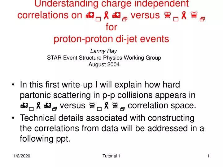
Understanding charge independent correlations on h 1 -h 2 versus f 1 -f 2 for proton-proton di-jet events. In this first write-up I will explain how hard partonic scattering in p-p collisions appears in h 1 -h 2 versus f 1 -f 2 correlation space.

E N D
Understanding charge independent correlations on h1-h2 versus f1-f2 forproton-proton di-jet events • In this first write-up I will explain how hard partonic scattering in p-p collisions appears in h1-h2 versus f1-f2 correlation space. • Technical details associated with constructing the correlations from data will be addressed in a following ppt. Lanny Ray STAR Event Structure Physics Working Group August 2004 Tutorial 1
Typical p-p collision producing two jets, more-or-less back-to-back: The jets are not exactly back-to-back due to differences between the parton momenta in each proton both along, and transverse to the beam direction. For simplicity I only consider two-jet events in this tutorial. jet proton parton- parton cm jet NN cm proton Other events may have back-to-back jets. In general observed jets will vary in pseudorapidity location as permitted by the acceptance. parton-parton cm is NOT same as NN cm proton proton Event A Event B NN cm NN cm proton proton Tutorial 1
Consider all pairs of particles in each event and compute the relative azimuth f1-f2 for each pair. Construct a histogram (shown below) of number of pairs on f1-f2. Note that we do not use a special trigger particle. Jet-A proton Parton cm Jet-B NN cm f proton Pairs of particles in which one particle is taken from one jet and the other particle is taken from the other jet have relatively large values of f1-f2 and contribute here: Pairs of particles within jet-A and within jet-B have relatively small values of f1-f2 and contribute here: A-B B-A A-A B-B Construct histogram using all pairs from all events. Number of pairs 0 p fD=f1-f2 Tutorial 1
Width of f1-f2 peaks at small and large relative azimuth: Number of pairs p 0 fD=f1-f2 Width of large angle peak is due to parton fragmentation cone plus any scatter away from 1800 in the relative azimuth angle between the “centroids” of the two jets in each event. Width of small relative angle peak reflects the angular width of the parton fragmentation process. Tutorial 1
Similarly, use all pairs of particles in each event and for each pair compute the relative pseudorapidity h1-h2. Construct a histogram (shown below) of number of pairs on h1-h2. Note that we do not use a special trigger particle. Jet-A proton parton-parton cm Jet-B NN cm h proton Pairs of particles in which one particle is taken from one jet and the other particle is taken from the other jet have finite positive or negative values of h1-h2 and contribute here or here: Pairs of particles from within Jet-A and from within Jet-B have relatively small values of h1-h2 and contribute here: A-A B-B A-B B-A This histogram is for the individual two-jetp-p collision event shown above Number of pairs h1-h2 0 Tutorial 1
h1-h2for pairs of particles from other two-jet events also produce peaks symmetric about 0 but at different positive and negative values. The peak at 0 due to pairs of particles taken within the same jet accumulates for all events. Event #1 Event #2 Event #3 -1 0 +1 Summing these individual event histograms over all events results in a strong peak at h1-h2 = 0 reflecting the average pseudorapidity width of all jets in the events. The peaks associated with pairs of particles from different jets are distributed across the full acceptance. hD=h1-h2 acceptance limit acceptance limit Number of pairs hD=h1-h2 -2 0 +2 Tutorial 1
0 p p 0 fD=f1-f2 -2 0 2 hD=h1-h2 Moving from 1D to 2D distributions… Next we plot the number of pairs in two-dimensional bins on hD=h1-h2 vs fD=f1-f2 for every pair of particles in every event. Large relative azimuth and uniform distribution on hD. large azimuth peak Small relative angles on both hD and fD. small angle peak Tutorial 1
So far I have only discussed making histograms of the number of particle pairs. For actual data analysis we must also account for the effects of detector acceptance, efficiency and single particle distributions. • In other words, what would the number of pair histograms look like in the absence of dynamics, but assuming the same single particle distributions and detector acceptance. • All of these effects are accounted for by dividing the pair number histograms, bin-by-bin, by analogous pair number histograms made from “mixed pairs” of particles taken from different but similar events. • The resulting ratio is closely related to two-particle correlations – the principal object of interest. • Correlation analysis details will be explained in another tutorial. Tutorial 1
Measured correlations in 200 GeV p-p collisions We are now ready to describe some real STAR data: Putting the preceding structures together on (h1-h2,f1-f2) and dividing by a mixed pair histogram produces the 2D histogram ratio landscape shown here. 0.85 < pt1 , pt2 < 2.3 GeV/c Large azimuth angle flat peak approximately independent of h1-h2 where: fD = f1-f2 hD = h1-h2 Small angle symmetric peak from parton fragmentation (plus quantum correlations for identical particles). Tutorial 1