Model-Checking Frameworks: Outline

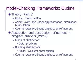
1. Model-Checking Frameworks: Outline • Theory (Part 1) • Notion of Abstraction • Aside: over- and under-approximation, simulation, bisimulation • Counter-example-based abstraction refinement • Abstraction and abstraction refinement in program analysis (Part 2) • Kinds of abstraction: • Data, predicate • Building abstractions • Aside: weakest precondition • Counter-example-based abstraction refinement

2. Outline, cont’d • 3-valued abstraction and abstraction-refinement (Part 3) • 3-valued logic • Theory of 3-valued abstractions: combining over- and under-approximation • 3-valued model-checking • Building 3-valued abstractions • Counter-example-based abstraction refinement

3. Acknowledgements The following materials have been used in the preparation of this lecture: • Edmund Clarke • “SAT-based abstraction/refinement in model-checking”, a course lecture at CMU • Corina Pasareanu • Conference presentations at TACAS’01 and ICSE’01 • John Hatcliff • Course materials from Specification and Verification in Reactive Systems Many thanks for providing this material!

4. Model Checking • Given a: • Finite transition system M(S, s0, R, L) • A temporal property φ • The model checking problem: • Does Msatisfy φ? ? M⊨φ

5. I Model Checking (safety) Add reachable states until reaching a fixed-point = bad state

6. I Model Checking (safety) Too many states to handle ! = bad state

7.      Abstraction S S’ Abstraction Function  : S ! S’

8. Abstraction Function: A Simple Example • Partition variables into visible(V) and invisible(I) variables. The abstract model consists of V variables. I variables are made inputs. The abstraction function maps each state to its projection over V.

9. Abstraction Function: Example x1 x2 x3 x4 0 0 0 0 0 0 0 1 0 0 1 0 0 0 1 1 x1 x2  0 0 Group concrete states with identical visible part to a single abstract state.

10. Computing Abstractions  S S’ • S – concrete state space • S’– abstract state space • : S→ S’- abstraction function • : S’ → S - concretization function • Properties of  and : • ((A)) = A, for A in S’ • ((C)) ⊇ C, for C in S • The above properties mean that  and  are Galois-connected 

11. Aside: simulations M = (s0, S, R, L) M’ = (t0, S’, R’, L’) Definition: p is a simulation between M and M’ if • (s0, t0) p •  (t, t1)  R’ (s, s1)  R s.t. (s, t) p and (s1, t1) p Intuitively, every transition in M’ corresponds to some transition in M

12. Aside: bisimulation M = (s0, S, R, L) M’ = (t0, S’, R’, L’) Definition: p is a bisimulation between M and M’ if • p is a simulation between M and M’ and • p is a simulation between M’ and M

13. Computing Existential Transition Relation • R[Dams’97]: (t, t1)  R’ iff  s (t) s.t.  s1  (t1) and (s, s1)  R • This ensures that M’ is the over-approximation if M, or M’ simulates M.

14. Abstract Kripke Structure • Abstract interpretation of atomic propositions • I ’(a, p) = true iff forall s in (a), I (s, p) = true • I ’(a, p) = false iff forall s in(a), I (s, p) = false • Abstract Transition Relation (2 choices) • Over-Approximation (Existential) • Make a transition from an abstract state if at least one corresponding concrete state has the transition. • Under-Approximation (Universal) • Make a transition from an abstract state if allthe corresponding concrete states have the transition.

15. Existential Abstraction (Over-Approximation) I I

16. K’ K Preservation via Over-Approximation • Let φbe a universal temporal formula (ACTL, LTL) • Let K’ be an over-approximating abstraction of K • Preservation Theorem • K’⊨φimpliesK ⊨ φ • Converse does not hold • K’⊭φ does not implyK⊭φ!!! • K’ may have extra behaviors

17. Computing Transition Relation • R[Dams’97]: (t, t1)  R’ iff  s (t)  s1  (t’) and (s, s1)  R • This ensures that M’ is the under-approximation if M, or M simulates M’.

18. Universal Abstraction (Under-Approximation) I I

19. K K’ Preservation via Under-Approximation • Let φbe an existential temporal formula (ECTL) • Let K’ be an under-approximating abstraction of K • Preservation Theorem • K’⊨φimpliesK ⊨ φ • Converse does not hold • K’⊭φ does not implyK⊭φ!!! • K’ may miss some behaviors

20. Which abstraction to use? But what about mixed properties?!

21. Our specific problem Let φbe a universally-quantified property (i.e., expressed in LTL or ACTL) and M’ simulates M • Preservation Theorem M’⊨φM ⊨ φ Converse does not hold M’⊭φM⊭φ The counterexample may be spurious

22. Checking the Counterexample • Counterexample : (c1, …,cm) • Each ci is an assignment to V. • Simulate the counterexample on the concrete model.

23. Checking the Counterexample Concrete traces corresponding to the counterexample: (Initial State <- s0 in our case) (Unrolled Transition Relation) (Restriction of V to Counterexample)

24. Abstraction-Refinement Loop Abstract Model Check Pass M, φ,  M’,φ No Bug Fail ’ Refine Check Counterexample Spurious Real Bug

25. Frontier φ Visible Invisible Inputs Refinement methods… Localization (R. Kurshan, 80’s)

26. Refinement methods… Abstraction/refinement with conflict analysis (Chauhan, Clarke, Kukula, Sapra, Veith, Wang, FMCAD 2002) • Simulate counterexample on concrete model with SAT • If the instance is unsatisfiable, analyze conflict • Make visible one of the variables in the clauses that lead to the conflict

27. Deadend states I I f Bad States Failure State Why spurious counterexample?

28. Refinement • Problem: Deadend and Bad States are in the same abstract state. • Solution: Refine abstraction function. • The sets of Deadend and Bad states should be separated into different abstract states.

29. ’ Refinement ’ ’ ’ ’ ’ ’ Refinement : ’

30. Deadend States Refinement

31. Deadend States Bad States Refinement

32. 1 0 0 1 0 0 1 0 0 1 0 0 1 1 1 0 1 0 1 1 Refinement as Separation Refinement : Find subset U of I that separates between all pairs of deadend and bad states. Make them visible. Keep U small ! d1 0 1 0 0 1 0 1 I b1 V b2

33. 0 1 0 1 0 1 0 0 1 0 0 1 0 0 1 0 0 1 1 1 0 1 0 1 Refinement as Separation Refinement : Find subset U of I that separates between all pairs of deadend and bad states. Make them visible. Keep U small ! d1 I b1 V b2

34. Refinement as Separation The state separation problem Input: Sets D, B Output: Minimal U  I s.t.:  d D,  b B, u U. d(u)  b(u) The refinement ’ is obtained by adding Uto V.

35. Two separation methods • ILP-based separation • Minimal separating set. • Computationally expensive. • Decision Tree Learning based separation. • Not optimal. • Polynomial. We will not talk about these in class