Download
1 / 11
120 likes | 248 Views
Introduction to Non Parametric Statistics Kernel Density Estimation. Nonparametric Statistics. Fewer restrictive assumptions about data and underlying probability distributions. Population distributions may be skewed and multi-modal. Kernel Density Estimation (KDE).

E N D
Introduction to Non Parametric Statistics Kernel Density Estimation
Nonparametric Statistics • Fewer restrictive assumptions about data and underlying probability distributions. • Population distributions may be skewed and multi-modal.
Kernel Density Estimation (KDE) Kernel Density Estimation (KDE) is a non-parametric technique for density estimation in which a known density function (the kernel) is averaged across the observed data points to create a smooth approximation.
Density Estimation and Histograms Let b denote the bin-width then the histogram estimation at a point x from a random sample of size n is given by, Two choices have to be made when constructing a histogram: • Positioning of the bin edges • Bin-width
KDE – Smoothing the Histogram Let be a random sample taken from a continuous, univariate density f. The kernel density estimator is given by, • K is a function satisfying • The function K is referred to as the kernel. • h is a positive number, usually called the bandwidth or window width.
Kernels • Refer to Table 2.1 Wand and Jones, page 31. • … most unimodal densities perform about the same as each other when used as a kernel. • Typically K is chosen to be a unimodal PDF. • Use the Gaussian kernel. • Gaussian • Epanechnikov • Rectangular • Triangular • Biweight • Uniform • Cosine Wand M.P. and M.C. Jones (1995), Kernel Smoothing, Monographs on Statistics and Applied Probability 60, Chapman and Hall/CRC, 212 pp.
KDE – Based on Five Observations Kernel density estimate constructed using five observations with the kernel chosen to be the N(0,1) density. x=c(3, 4.5, 5.0, 8, 9)
Histogram - Positioning of Bin Edges x=c(3, 4.5, 5.0, 8, 9) Area=1 • hist(x,right=T,freq=F), R-default • (a,b] right closed (left-open) • hist(x,right=F,freq=F) • [a,b) left closed (right-open)
Histogram - Bin Width hist(x,breaks=5,right=F,prob=T) hist(x,breaks=2,right=F,prob=T) Area=1
KDE – Numerical Implementation "kde" <- function(x,h) { npt=100 r <- max(x) - min(x); xmax <- max(x) + 0.1*r; xmin <- min(x) - 0.1*r n <- length(x) xgrid <- seq(from=xmin, to=xmax, length=npt) f = vector() for (i in 1:npt){ tmp=vector() for (ii in 1:n){ z=(xgrid[i] - x[ii])/h density=dnorm(z) tmp[ii]=density } f[i]=sum(tmp) } f=f/(n*h) lines(xgrid,f,col="grey") } #end function Variable description x = xgrid X = x
Bandwidth Estimators • Optimal Smoothing • Normal Optimal Smoothing • Cross-validation • Plug-in bandwidths