Download
1 / 27
270 likes | 283 Views
Statistical Data Analysis: Lecture 6. 1 Probability, Bayes’ theorem 2 Random variables and probability densities 3 Expectation values, error propagation 4 Catalogue of pdfs 5 The Monte Carlo method 6 Statistical tests: general concepts 7 Test statistics, multivariate methods

E N D
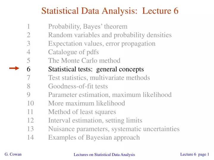
Statistical Data Analysis: Lecture 6 1 Probability, Bayes’ theorem 2 Random variables and probability densities 3 Expectation values, error propagation 4 Catalogue of pdfs 5 The Monte Carlo method 6 Statistical tests: general concepts 7 Test statistics, multivariate methods 8 Goodness-of-fit tests 9 Parameter estimation, maximum likelihood 10 More maximum likelihood 11 Method of least squares 12 Interval estimation, setting limits 13 Nuisance parameters, systematic uncertainties 14 Examples of Bayesian approach Lectures on Statistical Data Analysis
Example setting for statistical tests: the Large Hadron Collider Counter-rotating proton beams in 27 km circumference ring pp centre-of-mass energy 14 TeV Detectors at 4 pp collision points: ATLAS CMS LHCb (b physics) ALICE (heavy ion physics) general purpose Statistical methods for particle physics
The ATLAS detector 2100 physicists 37 countries 167 universities/labs 25 m diameter 46 m length 7000 tonnes ~108 electronic channels Statistical methods for particle physics
A simulated SUSY event in ATLAS high pT jets of hadrons high pT muons p p missing transverse energy Statistical methods for particle physics
Background events This event from Standard Model ttbar production also has high pT jets and muons, and some missing transverse energy. → can easily mimic a SUSY event. Statistical methods for particle physics
Statistical tests (in a particle physics context) Suppose the result of a measurement for an individual event is a collection of numbers x1 = number of muons, x2 = mean pt of jets, x3 = missing energy, ... follows some n-dimensional joint pdf, which depends on the type of event produced, i.e., was it For each reaction we consider we will have a hypothesis for the pdf of , e.g., etc. Often call H0 the signal hypothesis (the event type we want); H1, H2, ... are background hypotheses. Lectures on Statistical Data Analysis
Selecting events Suppose we have a data sample with two kinds of events, corresponding to hypotheses H0 and H1 and we want to select those of type H0. Each event is a point in space. What ‘decision boundary’ should we use to accept/reject events as belonging to event type H0? H1 Perhaps select events with ‘cuts’: H0 accept Lectures on Statistical Data Analysis
Other ways to select events Or maybe use some other sort of decision boundary: linear or nonlinear H1 H1 H0 H0 accept accept How can we do this in an ‘optimal’ way? What are the difficulties in a high-dimensional space? Lectures on Statistical Data Analysis
Test statistics Construct a ‘test statistic’ of lower dimension (e.g. scalar) Goal is to compactify data without losing ability to discriminate between hypotheses. We can work out the pdfs Decision boundary is now a single ‘cut’ on t. This effectively divides the sample space into two regions, where we accept or reject H0. Lectures on Statistical Data Analysis
Significance level and power of a test Probability to reject H0 if it is true (error of the 1st kind): (significance level) Probability to accept H0 if H1 is true (error of the 2nd kind): (1 - b = power) Lectures on Statistical Data Analysis
Efficiency of event selection Probability to accept an event which is signal (signal efficiency): Probability to accept an event which is background (background efficiency): Lectures on Statistical Data Analysis
Purity of event selection Suppose only one background type b; overall fractions of signal and background events are ps and pb (prior probabilities). Suppose we select events with t < tcut. What is the ‘purity’ of our selected sample? Here purity means the probability to be signal given that the event was accepted. Using Bayes’ theorem we find: So the purity depends on the prior probabilities as well as on the signal and background efficiencies. Lectures on Statistical Data Analysis
Constructing a test statistic How can we select events in an ‘optimal way’? Neyman-Pearson lemma (proof in Brandt Ch. 8) states: To get the lowest eb for a given es (highest power for a given significance level), choose acceptance region such that where c is a constant which determines es. Equivalently, optimal scalar test statistic is N.B. any monotonic function of this is just as good. Lectures on Statistical Data Analysis
Purity vs. efficiency — optimal trade-off Consider selecting n events: expected numbers s from signal, b from background; →n ~ Poisson (s + b) Suppose b is known and goal is to estimate s with minimum relative statistical error. Take as estimator: Variance of Poisson variable equals its mean, therefore → So we should maximize equivalent to maximizing product of signal efficiency purity. Lectures on Statistical Data Analysis
Why Neyman-Pearson doesn’t always help The problem is that we usually don’t have explicit formulae for the pdfs Instead we may have Monte Carlo models for signal and background processes, so we can produce simulated data, and enter each event into an n-dimensional histogram. Use e.g. M bins for each of the n dimensions, total of Mn cells. But n is potentially large, →prohibitively large number of cells to populate with Monte Carlo data. Compromise: make Ansatz for form of test statistic with fewer parameters; determine them (e.g. using MC) to give best discrimination between signal and background. Lectures on Statistical Data Analysis
Multivariate methods Many new (and some old) methods: Fisher discriminant Neural networks Kernel density methods Support Vector Machines Decision trees Boosting Bagging New software for HEP, e.g., TMVA , Höcker, Stelzer, Tegenfeldt, Voss, Voss, physics/0703039 StatPatternRecognition, I. Narsky, physics/0507143 Lectures on Statistical Data Analysis
Linear test statistic Ansatz: Choose the parameters a1, ..., an so that the pdfs have maximum ‘separation’. We want: ts g (t) tb large distance between mean values, small widths Ss Sb t → Fisher: maximize Lectures on Statistical Data Analysis
Determining coefficients for maximum separation We have where this becomes In terms of mean and variance of Lectures on Statistical Data Analysis
Determining the coefficients (2) The numerator of J(a) is ‘between’ classes ‘within’ classes and the denominator is → maximize Lectures on Statistical Data Analysis
Fisher discriminant Setting gives Fisher’s linear discriminant function: H1 Corresponds to a linear decision boundary. H0 accept Lectures on Statistical Data Analysis
Fisher discriminant: comment on least squares We obtain equivalent separation between hypotheses if we multiply the ai by a common scale factor and add an arbitrary offset a0: Thus we can fix the mean values t0 and t1 under the null and alternative hypotheses to arbitrary values, e.g., 0 and 1. Then maximizing is equivalent to minimizing Maximizing Fisher’s J(a) →‘least squares’ In practice, expectation values replaced by averages using samples of training data, e.g., from Monte Carlo models. Lectures on Statistical Data Analysis
Fisher discriminant for Gaussian data Suppose is multivariate Gaussian with mean values and covariance matrices V0 = V1 = V for both. We can write the Fisher discriminant (with an offset) as Then the likelihood ratio becomes Lectures on Statistical Data Analysis
Fisher discriminant for Gaussian data (2) (monotonic) so for this case, That is, the Fisher discriminant is equivalent to using the likelihood ratio, and thus gives maximum purity for a given efficiency. For non-Gaussian data this no longer holds, but linear discriminant function may be simplest practical solution. Often try to transform data so as to better approximate Gaussian before constructing Fisher discrimimant. Lectures on Statistical Data Analysis
Fisher discriminant and Gaussian data (3) Multivariate Gaussian data with equal covariance matrices also gives a simple expression for posterior probabilities, e.g., For a particular choice of the offset a0 this can be written: which is the logistic sigmoid function: (We will use this later in connection with Neural Networks.) Lectures on Statistical Data Analysis
Wrapping up lecture 6 We looked at statistical tests and related issues: discriminate between event types (hypotheses), determine selection efficiency, sample purity, etc. We discussed a method to construct a test statistic using a linear function of the data: Fisher discriminant Next we will discuss nonlinear test variables such as neural networks Lectures on Statistical Data Analysis