Download
1 / 28
290 likes | 424 Views
Beacon Vector Routing: Scalable Point-to-Point Routing in Wireless Sensornets. Presented by Jing Sun Computer Science and Engineering Department University of Conneticut. Geographic routing. +Highly scalable O(1) route discovery O(1) routing table

E N D
Beacon Vector Routing: Scalable Point-to-Point Routing in Wireless Sensornets Presented by Jing Sun Computer Science and Engineering Department University of Conneticut
Geographic routing • +Highly scalable • O(1) route discovery • O(1) routing table • Path lengths are close to the shortest path • -Each node should node its geographic coordinates • -Greedy forwarding can be suboptimal because it does not use real connectivity info.
Motivation for BVR • Simple – minimal complexity, with minimal assumptions about radio quality, presence of GPS, … • Scalable – low control overhead, small routing tables • Robust – node failure, wireless vagaries • Efficient – low routing stretch
Introduction of BVR – Cont. • 4 pieces • Deriving positions • Forwarding rules • Beacon Maintenance • Lookup: mapping node IDs positions • Used from other work: • Reverse path trees construction (Directed Diffusion) • Consistent hashing to map node identities to its current coordinates
Beacon-Vector: deriving positions • Randomly select nodes as beacons. The beacon vectors serve as coordinates • r beacon nodes (B0,B1,…,Br) flood the network; • P(q), a node q’s position, is its distance in hops to each beacon P(q) = B1(q), B2(q),…,Br(q) • k, p, C(k,p), Node p advertises its coordinates using the k closest beacons (we call this set of beacons C(k,p)) • Nodes know their own and neighbors’ positions • Nodes also know how to get to each beacon
Beacon-Vector: forwarding • Define the distance between two nodes P and Q as • To reach destination Q, choose neighbor to reduce distk(*,Q) • If no neighbor improves, enter Fallback mode: route towards the beacon which is closer to the destination • If Fallback fails, and you reach the beacon, do a scoped flood
Modeling The Forwarding Algorithm The sum of the differences for the beacons that are closer to the destination d than to the current routing node p The sum of the distances to the farther beacons We want to minimize:
Fallback towards B1 Example B1 B2 0,3,3 3,0,3 1,2,3 2,1,2 1,3,2 2,2,2 2,3,1 3,2,1 3,3,0 B3
Beacon maintenance • Route based on the beacons the source and destination have in common • Does not require perfect beacon info. • Each entry in the beacon vector has a sequence number • Periodically updated by the corresponding beacon • Timeout • If the #beacons < r, non-beacon nodes nominate themselves as beacons • Set a timer that is a function of its unique ID • If there’re more than r beacons • A beacon stop being a beacon if there’re more than r beacons with smaller IDs
Location directory • First look up the destination coordinates by name • Hashing H: nodeid → beaconid [14] • Use beacons as storage • Each node k that wants to be a destination periodically publishes its coordinates to its corresponding beacon bk = H(k) • When a node wants to route to node k, it sends a lookup request to bk • Cache the coordinates
Simulation Results • Assumptions for high level simulation • Fixed circular radio range • Ignore the network capacity and congestion • Ignore packet losses • Place nodes uniformly at random in a square planner region • 3200 nodes uniformly distributed in a 200 * 200 unit area • Radio range is 8 units • Vary #total beacons and #routing beacons
Success ratio given 10 routing beacons, node density per tx range
On-demand two hop neighbor acquisition • At lower densities, each node has fewer immediate neighbors • The performance of greedy routing drops • Add a neighbor’s neighbors to the routing table, if greedy forwarding is impossible
Performance under obstacles • Place horizontal & vertical walls with lengths of 10 or 20 units when the radio range is 8 units. BVR (True Positions)
Prototype evaluation • Office-Net: 42 mica2dot motes in a 20m * 50m office • Univ-Net: 74 mica2dot motes deployed across multiple student offices on a single floor in a UC Berkeley building
Questions? • Thank you!
Example Route from 3,2,1 to 1,2,3
Other Routing Protocols • Shortest Path • Scalability O(n2) message and O(n) routing state • Hierachical • Less message. O(nlogn) message and O(logn) message. • Maintainence issue. • Geographic Routing • O(1) and O(1) • Assumes fixed radio range • Require each node knows its geographic coordinates • Doesn’t consider real radio connectivity