Chapter 3 Best First Search

1. Chapter 3 Best First Search

2. Best First Search • So far, we have assumed that all the edges have the same cost, and that an optimal solution is a shortest path from the initial state to a goal state. • Let’s generalize the model to allow individual edges with arbitrary costs associated with them. • We’ll use the following denotations: length - number of edges in the path cost - sum of the edge costs on the path

3. Best First Search • Best First Search is an entire class of search algorithms, each of which employ acost function. The cost function: from a node to its cost. • Example: a sum of the edge costs from the root to the node. • We assume that a lower cost node is a better node. • The different best-first search algorithms differ primarily in their cost function.

4. Best First Search Best-first search employs two lists of nodes: • Open list • contains those nodes that have already been completely expanded • Closed list • contains those nodes that have been generated but not yet expanded.

5. Best First Search • Initially, just the root node is included on the Open list, and the Close list is empty. • At each cycle of the algorithm, an Open node of lowest cost is expanded, moved to Closed, and its children are inserted back to Open. • The Open list is maintained as a priority queue. • The algorithm terminates when a goal node is chosen for expansion, or there are no more nodes remaining in Open list.

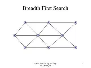
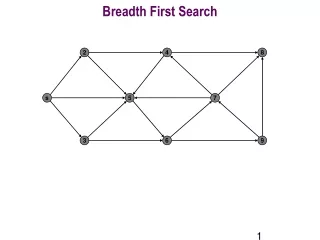
6. Example of Best First Search • One example of Best First Search is breadth first search. • The cost here is a depth of the node below the root. • The depth first search is not considered to be best-first-search, because it does not maintain Open and Closed lists, in order to run in linear space.

7. Uniform Cost Search • Let g(n) be the sum of the edges costs from root to node n. If g(n) is our overall cost function, then the best first search becomes Uniform Cost Search, also known as Dijkstra’s single-source-shortest-path algorithm . • Initially the root node is placed in Open with a cost of zero. At each step, the next node n to be expanded is an Open node whose cost g(n) is lowest among all Open nodes.

8. a 2 1 c b 2 1 2 1 e c f g c d c Example of Uniform Cost Search • Assume an example tree with different edge costs, represented by numbers next to the edges. Notations for this example: generated node expanded node

9. a 2 1 Example of Uniform Cost Search Closed list: Open list: a 0

10. a 2 1 c b 2 1 2 1 b c 2 1 Example of Uniform Cost Search Closed list: Open list: a

11. a 2 1 c b 2 1 2 1 e c d c a c b d e 2 2 3 Example of Uniform Cost Search Closed list: Open list:

12. 2 1 c b 2 1 2 1 e c f g c d c a c b d e f g 2 3 3 4 Example of Uniform Cost Search a Closed list: Open list:

13. a 2 1 c b 2 1 2 1 e c f g c d c a c b d e f g 3 3 4 Example of Uniform Cost Search Closed list: Open list:

14. a 2 1 c b 2 1 2 1 e c f g c d c a c b d e f g 3 4 Example of Uniform Cost Search Closed list: Open list:

15. 2 1 c b 2 1 2 1 e c f g c d c a c b d e f g 4 Example of Uniform Cost Search a Closed list: Open list:

16. a 2 1 c b 2 1 2 1 e c f g c d c a c b d e f g Example of Uniform Cost Search Closed list: Open list:

17. Uniform Cost Search • We consider Uniform Cost Search to be brute force search, because it doesn’t use a heuristic function. • Questions to ask: • Whether Uniform cost always terminates? • Whether it is guaranteed to find a goal state?

18. Uniform Cost Search - Termination • The algorithm will find a goal node or report than there is no goal node under following conditions: • the problem space is finite • there must exist a path to a goal with finite length and finite cost • there must not be any infinitely long paths of finite cost • We will assume that all the edges have a minimum non-zero edge cost e to a solve a problem of infinite chains of nodes with zero-cost edges. Then, UCS will eventually reach a goal of finite cost if one exists in the graph.

19. Uniform Cost Search - Solution Quality • Theorem 3.1 : In a graph where all edges have a minimum positive cost, and in which a finite path exists to a goal node, uniform-cost search will return a lowest-cost path to a goal node. • Steps of proof • show that if Open contains a node on an optimal path to a goal before a node expansion, then it must contain one after the node expansion • show that if there is a path to a goal node, the algorithm will eventually find it • show that the first time a goal node is chosen for expansion, the algorithm terminates and returns the path to that node as the solution

20. Uniform Cost Search - Time Complexity • In the worst case • every edge has the minimum edge e. • c is the cost of optimal solution, so once all nodes of cost c have been chosen for expansion, a goal must be chosen • The maximum length of any path searched up to this point cannot exceed c/e, and hence the worst-case number of such nodes is bc/e . • Thus, the worst case asymptotic time complexity of UCS is • O(bc/e )

21. Uniform Cost Search - Space Complexity • As in all best-first searches, each node that is generated is stored in the Open or Closed lists, and hence the asymptotic space complexity of UCS is the same as its asymptotic time complexity. • As a result, UCS is memory-limited in practice. The worst case asymptotic space complexity of UCS is O(bc/e )

22. Complexity of Dijkstra’s Algorithm • While Dijkstra’s algorithm is the same as uniform search, its time complexity is usually reported as n2. It is not a discrepancy, because: • n is the total number of nodes in the graph. In UCS we measure problem size by the branching factor b and solution cost c. • The Dijkstra’ algorithm it is assumed that every node may be connected to every node, which gives rise to the quadratic complexity. In UCS we assume a constant-bounded branching factor of b.

23. Combinatorial Explosion • All the problems we have seen so far are brute-force methods, i.e. they rely only on the problem space, the initial state and description of the goal state. • A brute-force algorithm can be expected to generate about a million sates per second. For example, the Fifteen Puzzle has 1013 would require about two month of computation, and 3 X 3 X 3 Rubik’s Cube would take about 686 thousand years. • The brute-force search algorithms are not efficient enough to solve even moderately large problems. A new idea is needed!

24. Heuristic Evaluation Functions • The efficiency of a brute-force can be greatly by the use of a heuristic static evaluation function, or heuristic function. • Such a function can improve the efficiency of a search algorithm in two ways: • leading the algorithm toward a goal state • pruning off branches that don’t lie on any optimal solution path.

25. Example of Heuristic Functions • Task :Navigating in a network of roads from one location to another Heuristic function: airline distance • Task :Sliding -tile puzzles Heuristic function: Manhattan distance - number of horizontal and vertical grid units a each tile is displaced from its goal position.Each tile must move at least Manhattan distance. • Task :Salesman Problem Heuristic function:A cost of minimum spanning tree(MST) of the cities

26. Properties of Heuristic Functions • The two most important properties of a heuristic function are: • it is a relatively accurate estimator of the cost to reach a goal. • it is relatively cheap to compute. • Another property : • admissibility - the heuristic function is always a lower bound on actual solution cost.

27. Pure Heuristic Search • Given a heuristic evaluation function, the simplest algorithm that uses it is: where f(n) - cost function h(n) - heuristic function This algorithm is called Pure heuristic search (PHS) • PHSwill eventually generate the entire graph finding a goal node if one exists. • If the graph is infinite, PHS is not guaranteed to terminate, even if a goal node exists. f(n) = h(n)

28. s 1 3 b a 2 1 g Pure Heuristic Search • If the PHS terminates with solution, it is not guaranteed to be an optimal one. • Example: Here the algorithm will return a solution of length 4, when one of length 3 exists. The problem is that PHS only considers the estimated cost h(n) to a goal when choosing a node for expansion, and doesn’t consider the cost g(n) from the initial state to the node. Path returned (not optimal)

29. In order to find optimal solution, we have to take into account the cost of reaching each Open node from the initial state, as well as the heuristic estimate of remaining cost s to goal. when Wh/Wg = W, 1<W< The Heuristic Searches Family f(n) = Wg g(n) + Wh h(n) This table presents results of research of the Heuristic Searches family. We can clearly see that while a path length changes linearly, the number of expanded nodes grows exponentially.

30. A* Algorithm • We take into account both the cost of reaching a node form the Initial state, g(h), as well as the heuristic estimate from that node to the goal node, h(n). • For given h(n), this is the best estimate of a lowest cost path from the initial state to a goal state that is constrained to pass through node n • The a stands for “algorithm”, and the * indicates its optimality property. f(n) = g(n) + h(n)

31. A* - Terminating Conditions • Like all best-first searches, A* terminates when it chooses a goal node for expansion, or when there are no more Open nodes. • In a finite graph, it will explore the entire graph if it doesn’t find a goal state. • In an infinite graph it will find a finite-cost path if • all edge costs are finite and have a minimum positive value • all heuristic values are finite and non-negative. • Under those conditions the cost of nodes will eventually increase without bound. Therefore, there could not be an infinite loop.

32. s 1 1 b a 2 1 c A* - Solution Quality • In general, A* is guaranteed to return optimal solutions. • Example: • The problem in this example is that the heuristic value at node b (3) overestimates the cost of reaching a goal from node b, which is only 1. h(b)= 3 f(b) = 1 + 3 = 4 h(a )= 1 f(a) = 1 + 1 = 2 h(c)= 0 f(c) = 3 + 0 = 3 Path returned (not optimal)

33. A* - Solution Quality • Theorem 3.2 : In a graph where all edges have a minimum positive cost, and non-negative heuristic values that never overestimate actual cost, in which a finite-cost path exists to a goal state, A* will return an optimal path to a goal. • Steps of proof • show that if Open contains a node on an optimal path to a goal before a node expansion, then it must contain one after the node expansion • show that if there is a path to a goal node, the algorithm will eventually find it • show that the first time a goal node is chosen for expansion, the algorithm terminates and returns the path to that node as the solution.

34. Admissible, Consistent and Monotonic Heuristics • Admissible: if we define h*(n) as the exact lowest cost from node n to a goal, a heuristic function h(n) is admissible if and only if n • Consistent: this quality is similar to the triangle inequality of all metrics. If c(n,m) is the cost of a shortest path from node n to node m , then a heuristic function h(x) is consistent if n,m h(n)  h*(n) h(n)  c(n,m) + h(m)

35. Admissible, Consistent and Monotonic Heuristics • Monotonic: If a heuristic function h(n) is consistent, then the cost function f(n) is monotonic nondecreasing,i.e if and only if for all children n’ of n , • Proof: h(n) c(n,n’)+h(n) g(n) + h(n)  g(n)+c(n,n’) + h(n’) g(n) + h(n)  g(n’) + h(n’) f(n)  f(n’) Applying the same proof in the opposite direction shows that monotonicity of implies consistency of h. Thus, the two properties are equivalent. f(n)  f(n’)

36. Admissible, Consistent and Monotonic Heuristics • Consistency implies admissibility To see this, we replace m with a goal node G. • Proof: h(n) c(n,m)+h(m) h(n)  c(n,G) + h(G) h(G) = 0 h(n)  c(n,G) (the shortest path) h(n)  h*(n) • Admissibility does not imply consistency.Consistency is a stronger property.

37. Admissible, Consistent and Monotonic Heuristics • Given an admissible but inconsistent function h (which is rare), we can easily construct a monotonic f function that is still admissible: • whenever the f(n’) value of a child node n’ is less the the f(n) value of its parent node n, we set he f(n’) value of the child to the f(n) value of the parent • if the heuristic function h(n) is admissible, the the new cost function f(n) will also be admissible, as follows. If h(n) is a lower bound on the cost of reaching the goal , then f(n) = g(n) +h(n) is a lower bound on total cost of reaching the goal from the initial state via the current path. Therefore, the total cost of reaching the goal via every child of node n must be at least as large as the minimum cost though the parent. • f(n’’) = max(f(n’), f(n))

38. Time Complexity of A* • The running time of A* is proportional to the number of nodes generated or expanded.Therefore the branching factor is at most a constant, and heuristic evaluation of a node can be done in constant time. • The Open and Closed lists can be maintained in constant time per node expansion. • Closed list - can be organized as hash table, since we only need to check for the occurrence of a node. • Open list - we have to be able to insert a node and retrieve a lowest-cost node in constant time. This wold take time that is logarithmic in the size of the Open list. • In many cases, the heuristic functions and edge costs are integer valued or have a small number of distinct values. In such case, the Open can be maintained as an array of lists, separate list for each different cost. This allows constant-time insertion and retrieval from the Open list. Thus, the question is how many nodes A* generates in the process of finding a solution. The answer depends on the quality of the heuristic function.

39. Special Cases • Worst case: Cost function f(n) = g(n) • the heuristic function returns zero for every node and provides no information to the algorithm, but is still a lower-bound on actual cost.This is identical to the UCS or Dijkstra’s algorithm, which has a worst-case time complexity of • Best case: Cost function f(n) = g(n) + h*(n) • the heuristic function is perfect and always returns the exact optimal cost to a goal state from any given state,The optimal path will be chosen, and the number of node-expansion cycles will be d( the depth of the optimal path. Thus, the asymptotic time complexity is O(bc/e ) O(bd) = O(d)

40. Tie Breaking • Example h(b)= 2 f(b) = 1 +2 = 3 s h(b)= 2 f(b) = 1 +2 = 3 1 1 b a 2 2 2 2 g1 g2 c g3 c g4 c h(b)= 1 f(b) = 2 +1 = 3

41. Tie Breaking • Consider a problem where every node at depth d is a goal node, and every path to depth d is and optimal solution path. As such a tree is explored, every node will have the same cost. If ties are broken in favor of nodes with lower g costs the entire tree may be generated before a goal node. Thus, the asymptotic time complexity would be O(bd), in spite of the fact that we have a perfect heuristic function.

42. Tie Breaking • A better tie breaking rule is to always break ties among nodes with the same f(n) value in favor of nodes with the smallest h(n) value (or the largest g(n) value). This ensures that: • any tie will always be broken in favor of a goal node, which has h(G) = 0 by definition. • the time complexity of A* with a perfect heuristic will be O(d).

43. Conditions for Node Expansion by A* • If the heuristic function is consistent, then the cost function f(n) is nondecreasing along any path away from the root node. The sequence of nodes expanded by A* starts a the h(s) and stays the same or increases until it reaches the cost of an optimal solution. Some nodes with the optimal solution cost might be expanded, until a goal node is chosen.

44. Conditions for Node Expansion by A* • This means that all nodes n whose cost f(n) < c will certainly be expanded, (where c is optimal solution cost), and no nodes n whose cost f(n) > c will be expanded. Some nodes n whose cost f(n) = c will be expanded. Thus, f(n) < c is a sufficient condition for A* to expand node n, and f(n)  c is a necessary condition.

45. Time optimality of A* • Theorem 3.3 : For a given consistent heuristic function, every admissible algorithm must expand all nodes surely expanded by A*. • Proof Suppose that there exists an admissible algorithm B, a problem P, a consistent heuristic function h and a node m such that node m is not expanded by algorithm B on problem P with heuristic function h, but node m is surely expanded by A*, meaning that f(m) = g(m) + h(m) < c. Let’s construct a new problem P’ that is identical to problem P, except for the addition of a single new edge leaving node m, which leads to a new goal nodes z. Let the cost of the edge from node m to node z be h(m), the heuristic value of node m in problem , or c’(m,z) = h(m). We use c’(m,x) here to denote the actual cost from m to z in problem P’. In problem P’, the cost of an optional path from the initial state to the new goal state is g(m) + c’(m,z) = g(m) + h(m) = f(m), since every path to z must go through node m. Since f(m) < c, the cost of an optimal solution to problem P, the optimal solution to problem P’ is the path from the start through node m to goal z. When we apply algorithm B to problem P’.By assumption, B never expands node m on problem P, thus it must not expand node m on problem P’ either. Thus B must fail to find the optimal solution to problem P’. Contradiction !

46. Space complexity of A* • The main drawback of A* is its space complexity. • Like all best-first search algorithms’ it stores all the nodes it generates in either the Open list or the Closed list.Thus, its space complexity is the same as its time complexity, assuming that a node can be stored in a constant amount of space. • On current computers, it will typically exhaust the available memory . • This algorithm is memory- limited.

47. The WA* Heuristics Family • A generalized version of A* Where: when Wh/Wg = W, 1<W< When W=1 it is A* When q= it is Pure Heuristic Search f(n) = Wg g(n) + Wh h(n) This table presents results of research of WA* for different values of W. We can clearly see that while a path length changes linearly, the number of expanded nodes grows exponentially.

48. Appendix 1 Abstract Analysis

49. Abstract Analytic model • We assume that • the problem space is a tree, with no cycles. • there is a uniform branching factor b, meaning that every node has b children • every edge or operator costs one unit to apply. • there is a single goal node at depth d in the tree • The impact of this assumption is that once we diverge from the optimal path from the root to goal, the only way to reach the goal is to backtrack until we rejoin the single optimal path.

50. We assume that the heuristic function is that it has constant absolute error. It means that it never underestimates he optimal cost of reaching a goal by more than a constant. Thus, for some constant k We need to determine how many nodes will be expanded under these assumptions. Consider a node n in the tree.Assume that the path from the start node s to node n diverges from the path to the goal at node m. Let d to be a distance from s to g , x to be the distance from s to m, and y the distance from from m to n. Thus: h*(n) = y + (d -x) h(n) = y + d - x - k f(n) = g(n) + h(n) = x+ y +y +d - x -k = 2y + d - k  d y  k/2 Constant Absolute Error h(n) = h*(n) - k