LONG WAVE RADIATION AT SEA SURFACE

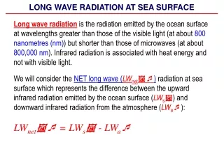
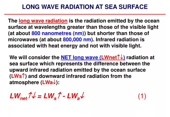
1. LONG WAVE RADIATION AT SEA SURFACE Thelong wave radiation is the radiation emitted by the ocean surface at wavelengths greater than those of the visible light (at about 800 nanometres (nm)) but shorter than those of microwaves (at about 800,000 nm). Infrared radiation is associated with heat energy and not with visible light. We will consider the NET long wave (LWnet) radiation at sea surface which represents the difference between the upward infrared radiation emitted by the ocean surface (LWs) and downward infrared radiation from the atmosphere (LWa): LWnet = LWs - LWa(1)

2. Net LW radiation at sea surface comes out as a result of many complex processes LWnet=???

3. The ocean surface irradiance consists of the emitted LW radiation from the sea surface and reflected atmospheric LW irradiance: LWs = LWs0 + LLWa (2) where LWs0 is LW irradiance of ocean surface L is surface long wave albedo Thus, the net LW radiation at sea surface can be expressed as: LWnet = LWs0 - (1-L)LWa (3)

4. Restaurant Two industrial workers go for a lunch: They take (besides the meals) each cup of tea simultaneously. • The first worker puts sugar into the cup immediately and starts to eat the main dish. • The second worker first starts to eat and puts the sugar into the cup just before the drinking. They start to drink their tea simultaneously Whose tea will be hotter at the moment of drinking?

5. Upward long wave irradiance from sea surface This is the major component of longwave exitance!!!!For this part the physics is a simple blackbody radiation LWs0 = Ts4(4) where is the Stefan-Boltzmann constant (5.6710-8Wm-2K-4) Tsis the sea surface !!!skin!!! temperature in degrees Kelvin  is the emissivity of the sea surface Emissivity of the sea surface in a general case depends on the sea state and optical properties of the sea water. For the fresh water  = 0.92and varies from 0.89 to 0.98 for different conditions.

6. Sea surface skin temperatureTs is not equivalent to SST, measured at ships by buckets or engine intakes, it is the temperature of very thin (several to several hundreds ) surface skin layer, namely skin temperature. Longwave absorption and emission both take place in just about the top 0.5 mm of water, depending on wavelength. Back to the skin temperature issue - later Downward amospheric long wave irradiance Downwelling longwave radiation (longwave irradiance) originates from the emission by atmospheric gases (mainly water vapor, carbon dioxide and ozone), aerosols and clouds. Long-wave albedo is also poorly known and depends on the sea state and cloud conditions. Downwelling LW is the smallest, but the most uncertain term in the net LW radiation (longwave exitance).

7. Determining surface net long wave radiation Measurements Modelling - RTMs Parameterization

8. Measurements of LW radiation: The pyrgeometer is of a similar construction to the pyranometer, but the single dome is made from silicon or similar material transparent to the longwave band, coated on the inside with an interference filter to block shortwave radiation. The longwave irradiance passing through the dome, which we wish to determine, is only one component of the thermal balance of the thermopile. The remaining components come from various parts of the instrument. To isolate the geophysical component, the manufacturers provide the correction equations.

9. More detailed description of pyrgeometer The PIR, or pyrgeometer, is sensitive to wavelengths in the range from 3000 to 50000 nm, which covers the span of temperatures (or thermal radiation) expected from the earth and atmosphere. The pyrgeometer works on the same principle as the pyranometer in that radiant energy is converted to heat energy which, in turn, is measured by a thermopile. However, protecting the sensor from the environment (e. g., solar radiation) is difficult. To do this, the dome is made of silicon, which is nearly opaque to solar wavelengths. The dome is also coated with a grayish interference filter that does not transmit wavelengths shorter than 3000 nm, but sharply increases to 50% transmission at 4000 nm. From 4000 to 50000 nm its transmittance slowly falls to about 30-40%. The detector senses a net signal from a number of sources which includes emissions from targets in its field of view, emission from the case of the instrument, and emission from the dome. To resurrect the true environmental thermal infrared irradiance, temperatures of the detector, case, and dome are monitored with thermistors. Because the case is shielded from the sun, its temperature represents the air temperature and therefore is a proxy for the degree of thermal emission by the atmosphere. The dome, however, is not protected from solar heating. Therefore, the difference between the thermal emissions of the case and dome represents an erroneous signal that must be removed. (As mentioned before, shading the dome would make this error negligible.) An empirical calibration equation accounts for all of these effects and converts the three measured temperatures to a true environmental thermal infrared irradiance in watts per square meter. Requirements for calibration facilities Calibrating facilities for infrared instruments are more complicated and therefore less common than those for solar radiation, and require careful technique. Field intercomparisons if several instruments are available are desirable. The use of on-site atmospheric soundings in clear-sky conditions can provide an absolute reference for longwave irradiance. The calculation of the downwelling longwave flux under a cloud requires knowledge of both cloud base height and emissivity. Cloud base height may be measured with active systems such as a MicroPulse lidar (Spinhirne, 1993) or a cloud profiling radar, although an infrared radiometer (such as the pyrgeometer) would still be needed to estimate cloud emissivity.

10. Modelling of the long wave radiation (RTMs) The radiative transfer equation (RTE) states that the energy radiated by a parcel of material in a particular frequency range and particular direction (denoted by an increment of solid angle around the direction) is the sum of energy transmitted through the parcel and the energy emitted from within the parcel, in that frequency interval and direction. RTE evaluates the effect of changes in temperature, humidity, cloud, aerosols, and chemical composition. Calculation of LW radiation should include all the major absorption bands of CO2, H2O, and O3, as well the weaker bands of CO2, N2O and CH4. Structure of a simple RTM Atmospheric column consists ofNplane parallel layers,n=1,2,…,N. TemperaturesTn, n=0,1,….,Nare denoted at layer edges. The mean optical thickness of thenthlayer at a particular frequencyisn.

11. At frequency  and beam angle  the upward IR irradiance U,n and the downward IR irradiance D,n at the edges of the layer n are: (5.6) where  = cos. In (5,6): the first terms are the transmitted IR irradiances given by Lambert’s law, and the second terms are the IR irradiances emitted in the layer: (7,8) whereB,nis the Planck function at frequencyand temperatureTn. Boundary conditions: (9,10) is the albedo, =1-is the emissivity of the ocean surface. Equation (9):no downward IR flux at the top of the atmosphere. Equation (10):the upflux at the ocean surface is given by the sum of emission from the ocean plus the reflection of the downward flux.

12. For the frequency range[a,b]the total upwardUnand downwardDnIR fluxes result from integratingU,nandU,noverall frequencies in[a,b]and beam angles: 9,10 • Problems: • Numerical solution of (5)-(12) is difficult and expensive due to: • The spectral complexity of the atmospheric constituents • Vertical inhomogeneity of the chemical composition of the • atmosphere • There is a lack of measurements of basic parameters in the atmospheric column

13. Short summary: Most exact are the Line-By-Line Radiative Transfer Models (LBLRTM) which compute transfer of each constituent for each emission and absorption spectral line at many levels throughout the profile. Their computational burden is therefore large, which makes them unsuitable for routine use in numerical models. Over the years therefore, many broadband RTM's have been developed, increasing in accuracy and efficiency with improved parameterizations and increased computer power. Such models are widely applied in climate modelling, and in flux retrieval from direct and remotely sensed atmospheric variables. The computation of LW flux with the best high spectral resolution codes under clear conditions is at an advanced state. For cloudy sky conditions, however, RTM's are not well validated. The calculation of the downwelling longwave flux under a cloud requires knowledge of both cloud base height and emissivity.

14. Parameterization of LW radiation: LWnet = LWs0 - (1-L)LWa What do we measure? SST Ta, q, C (Cn, Cl) 1. No problem to parameterize the LWs0 , if we have SST and the emissivity of the sea surface: LWs0 = Ts4 However, you have to remember that is Ts4 a skin temperature and is not equal to the bulk SST (LATER!)

15. 2. LW albedois more poorly known that a SW albedo. Some very tentative estimates give values in the range of 0.04-0.05 (e.g. Clark et al. 1974). Since • the value [1-LW albedo] is close (at least of the same • order as) to the emmissivity of sea surface [] • the accuracy ofLand is approximately the same • there is an approach to establish an effective emissivity and to re-write the equation for the net LW as follows: LWnet = Ts4 - (1-L)LWa LWnet = (Ts4 - LWa) (13) where is an effective emissivity and should not be understood as an emissivity of the sea surface (typical mistake). From (2), (4), (13):  =(LWs0 - LWa)/ (Ts4- LWa) (14) Important:   = LWs0 / Ts4

16. 3. Parameterization of downwelling atmospheric LW radiation LWnet = (Ts4- LWa) The simplest approach is to measure downwelling LW radiation and to compare it with different combinations of surface parameters: Tair, q, Cn, Cl However, this approach results in very uncertain dependencies due to very different optical properties of clear sky and cloudy atmosphere. Air temperature blackbody radiation shows significant differences for clear skies and cloudy skies.

17. Guest (1998) – 2 months of direct LW measurements in Weddell Sea: Cloudy conditions Clear sky Processes are quite different under clear skies and clouds ! separate analysis should be performed for atmospheric LW under clear sky and clouds

18. 1. Downwelling long wave radiation under clear skies Since information about atmospheric gases and aerosols is generally unavailable in routine observational practice, major efforts of researchers were concentrated on studying relationships between the clear sky downwelling atmospheric LW on • Surface humidity • Surface air temperature Theoretically, from a physical view point, surface humidity should have a closer link with surface humidity. Bignami et al. (1995) using results from direct observations in seven cruises in Mediterranean Sea, found close relationship between surface water vapor pressure and the ratio between atmospheric downwelling LW and air temperature blackbody radiation: LWa = Ta4(a+be) where a=0.684, b=0.0056, =0.75

19. However, in practice much better relationships are observed for surface air temperature. Reasons: • more easily available (more observations) • measurements are more accurate Swinbank (1963) from Indian Ocean and lake observations: LWa = Ta4(a+bTa)(14a) or ln(LWa / Ta4) =a+ln(Ta)(14b) where a=-15.75, =0.75 Guest (1998) tested many formulations of clear sky atmospheric LW.  No evidence of a better approximation for humidity than for air temperature.

20. Guest (1998) results (for your files):

21. Malevsky et al (1992) from a very big data set collected in different World Ocean regions (incl. tropics and mid-latitudes) found the following relationship between the downwelling atmospheric LW and humidity (water vapor pressure): LWa = Ta4(0.60+0.049e)(16) Similar dependency for air temperature was: LWa = 1.026Ta210-5 –0.541 (17) There has been found considerably lesser scatter for (17) than for (16) and a smaller RMS error. INTERESTING: equation (17) looks physically less reasonable than those which include Ta4. However, analysis of empirical data shows that formula (17) works well in most conditions.

22. Thus, now we assume the following form of parameterization of the net LW radiation: Sea surface !skin! temperature blackbody radiation. Since we do not have normally “skin” estimate, we account for the bulk effect in  Effective emissivity of sea surface (accounts for the LW albedo and skin effect) !!! LWnet = [ Ts4- ( LWa0 F(c) )] ? Atmospheric downwelling LW under clear skies: Parameterized as a function of either surface humidity or surface temperature Relationships with temperature give better results! Function of cloud cover – Should account for the effect of clouds

23. 2. Downwelling long wave radiation under clouds – the cloud modification of LWa. What should be parameterized from a theoretical view point is a cloud temperature blackbody radiation: Tcl4 Lind and Katsaros (1982): LWc(2) = n(2)(2) Tcl(2)4 + [1-n(2)] LWc(3) LWc(1) = n(1)(1) Tcl(1)4 + [1-n(1)] LWc(2) LWc(tot) = (1-(0)) LWc(1) + + LWa(sky) +(0)T0(1)4 nis fractional cloud cover of the subscribed cloud layer Tclis cloud base temperature of the subscribed cloud layer • is effective emittance of the • subscribed cloud layer • (0) is emittance of layer from the surface • to lowest cloud base Tclis equivalent radiative temperature of the lower layer We DO NOT know (measure) We come actually to another RTM!

24. LWa LWa + LWcl The only available parameter is the total fractional cloud cover and sometimes is the fractional cover of the low-level cloudiness. Typical approach: to make measurements under the known cloud conditions and to compare clear sky atmospheric LW with that measured under the cloudy sky. Paramete- rization of F(n) Bignami et al. (1995): F(n) = 1+0.1762c2 (Mediterranean Sea) Clark et al. (1974): F(n) = 1-0.69c2 (Pacific Ocean) Efimova (1962): F(n) = 1-0.80c (land data) Typical expression is 1ac for the total cloud cover This effect has to be parameterized

25. Malevsky et al. (1992) from his collection of field measurements for the total cloud cover found: LWcl+a = 0.928Ta210-5 –0.397 (18) He assumed that LWcl+a = LWa (1+ktnt2) (19) Coefficientktcan be derived from (19) under nt=1: kt = (LWcl+a + LWa) / (LWa)(20) where:LWa = 1.026Ta210-5 –0.541) Not surprisingly, in this formulationktbecomes dependent on the air temperature, since bothLWcl+aandLWaare the functions of air temperature.

26. Computation of the kt from a simple RTM: kt = (1/LWa) [cla Tcl4 + +LWa(0)(4h/Ta)-1] cl– emissivity of the cloud base cl– temperature of the cloud base LWa(0) – irradiance below the cloud layer cl– surface temperature  - temperature gradient in the undercloud layer h – cloud layer height Thus, for the total cloud cover only: LWa = [LWa0 F(c)]=(1.026Ta210-5-0.541)(1+ktnt2) kt = (-0.098Ta210-5 + 0.144) / (1.026Ta210-5-0.541)

27. Malevsky et al. (1992) first considered the effect of cloudiness for three different layers (low cloudiness, mid-level cloudiness and upper layer cloudiness). For upper layer:LWclu+a = 0.995Ta210-5 –0.496(21) For mid-level:LWclm+a = 0.932Ta210-5 –0.401(22) For lower layer:LWcll+a = 0.921Ta210-5 –0.385(23) For the cloud coefficients: For upper layer: ku = (LWclu+a+LWa)/(LWa)(24) For mid-level:km = (LWclm+a+LWa)/(LWa)(25) For lower layer:kl = (LWcll+a+LWa)/(LWa)(26)

28. However, normally we have observations only for the fractional cloud cover of total and low-layer cloudiness. Thus, this 3-layer formulation has been simplified for the consideration of the total and low-layer cloudiness: LWa = (1.026Ta210-5-0.541)(1+klnl2)(1+ku+m(nt2-nl2) (27) ku+mis the coeeficient accounting for the total effect of the mid and upper layer cloudiness, which can be derived from the coefficients for the total and low-level cloudiness: kl = (LWcll+a+LWa)/(LWa)(28) ku+m = (ktnt2 -klnl2) / [(1+ktnt2)(nt2–nl2)] (29) Now we can finally derive the parameterization of the net long-wave radiation at ocean surface in a general form: LWnet =  [Ts4 - (LWa0 F(c))]

29. Summary: • History is very long • The number of parameterizations approaches several tens • Formulations are similar • Differences are large

30. Variations in short-wave radiation and long-wave radiation due to the parameterizations (North Atlnatic SW and LW radiation budget)

31. Summary of LW radiation parameterizations: • Under clear sky and small cloudiness the accuracy is • normally better than 15 W/m2 • Higher uncertainties occur under the moderate and high • cloud cover • Uncertainties in the tropics are typically higher than in • mid and high latitudes and are primarily associated with • atmospheric clear sky IR irraidance • “Hot issues” of all parameterizations are “skin • temperature” and representation of the multi-layer • cloudiness of different types by fractional [total] cloud • cover

32. Recommendations: • Do not hesitate to use “old” parameterizations • Try to avoid the use of parameterizations based on water • vapor pressure and humidity • Do not use Bignami et al. (1995) except for Mediterranean • sea • Be careful with the choice of emissivity value. Always • remember – it is effective emissivity and not the • emissivity of surface

33. At the ocean surface: Incoming radiation surplus defcit Outgoing radiation At the top of atmosphere Radiation balance of the ocean RB = SW(1-) - LWnet(30) LW SW Winter SpringSummerFall

34. SW LW RB

35. Variations of SW and LW radiation due to different parameterizations

36. /helios/u2/gulev/handout/ • longwave1.f – collection of LW radiation F77 codes • RIZL – Malevsky et al. (1992) scheme • RLWISI – Efimova (1961) as modified by Isemer et al (1989) • RLW_CLA – Clark et al. (1974) • RLW_BIG – Bignami et al. (1995) • Try to compare Malevsky, Efimova, Bignami and Clark schemes: • For Ts = 12C: • Clear sky, dependence on temperature, humidity • Cloud cover octa=4, dependence on temperature • Tair = 15C, dependence on cloud cover (in octas)

37. /helios/u2/gulev/handout/ swm_test.f– program to compute instantaneous values of SW radiation, using Malevsky et al. (1992) and Dobson and Simth (1988) schemes. Compilation:f77 –o swm_test swm_test.f radiation.f • Results: sw.res • swr_test.f– program to compute daily values of SW radiation, using Reed (1977) scheme. • Compilation:f77 –o swr_test swr_test.f radiation1.f • Results: swr.res • lw_test.f – program to compute values of LW radiation, using Malevsky et al. (1992), Clark et al. (1974), Bignami et al. (1995) and Emivova (1962) schemes. • Compilation:f77 –o lw_test lw_test.f longwave1.f Results: lw.res

38. READING Angström, A.K., 1925: On the variation of the atmospheric radiation. Gerlands. Beitr. Geophys., 4, 21-145. Bignami, F., R.Santorelly, M.E.Schiano, and S.Marullo, 1991: Net long-wave radiation in the western Mediterranean Sea. Poster session at the 20th General Assembly of the International Union of Geodesy and Geophysics, IAPSO, Wien, August 1991. Bignami, F., S.Marullo, R.Santorelly, and M.E.Schiano, 1995: Long-wave radiation budget in the Mediterranean Sea. J. Geophys. Res.,100, 2501-2514. Brunt, D., 1932: Notes on radiation in the atmosphere. Quart. J. Roy. Met. Soc., 58, 389-420 Bunker, A., 1976: A computation of surface energy flux and annual cycle over the North Atlantic Ocean. Mon. Wea. Rew., 104, 1122-1140. Clark, N.E., L.Eber, R.M.Laurs, J.A.Renner, and J.F.T.Saur, 1974: Heat exchange between ocean and atmosphere in the eastern North Pacific for 1961-71. NOAA Tech Rep. NMFS SSFR-682, US Dept. of Commer., Washington DC, 108 pp. Efimova, N.A., 1961: On methods of calculating monthly values of net long-wave radiation. Meter. Hydr. 10, 28-33. Fung, I. Y., D.E.Harrison, and A. A. Lacis, 1984: On the variability of the net long-wave radiation at the ocean surface. Rev. Geophys., 22(2), 177-193. Gulev, S.K., 1995: Long-term variability of sea-air heat transfer in the North Atlantic Ocean. Int.J.Climatol., 15, 825-852. Isemer, H.-J., J.Willebrand, and L.Hasse, 1989: Fine adjustment of large-scale air-sea energy flux parameterizations by direct estimates of ocean heat transport. J.Climate, 2, 1163-1184. Josey, S., E.C.Kent, and P.K.Taylor, 1999: New insights into the ocean heat budget closure problem from analysis of the SOC air-sea flux climatology. J. Climate, 12, 2856-2880. Lind, R.J., K.B.Katsaros, and M.Gube, 1984: Radiation budget components and their parameterization in JASIN. Quart. J. Roy. Meteor. Soc., 110, 1061-1071. Lindau, R., 2000: Climate Atlas of the Atlantic Ocean derived from the Comprehensive Ocean-Atmosphere Data Set. Springer-Verlag, Berlin, 488 pp. Malevsky, S.P., G.V.Girdiuk, and B.Egorov, 1992b: Radiation balance of the ocean surface. Hydrometizdat, Leningrad, 148 pp. Oberhuber, J.M., 1988: An Atlas based on the COADS data set: the budgets of heat, buoyancy and turbulent kinetic energy at the surface of the global ocean. MPI fuer Meteorologie report, No. 15, 19pp. [Available from Max-Plank-Institute fuer Meteorologie, Bundesstrasse 55, Hamburg, Germany]. Rosati, A. and K. Miyakoda, 1988: A general circulation model for the upper ocean circulation. J. Phys. Oceanogr., 18, 1601-1626.