Eye fitting: Sensitivity to bumps

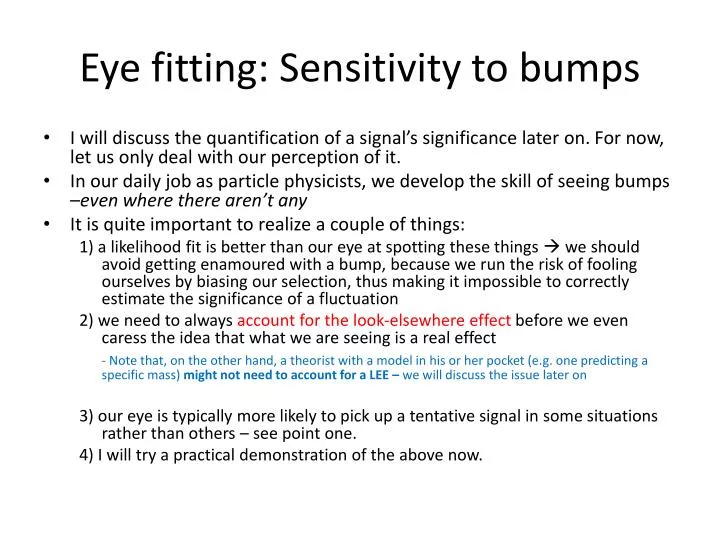
1. Eye fitting: Sensitivity to bumps • I will discuss the quantification of a signal’s significance later on. For now, let us only deal with our perception of it. • In our daily job as particle physicists, we develop the skill of seeing bumps –even where there aren’t any • It is quite important to realize a couple of things: 1) a likelihood fit is better than our eye at spotting these things  we should avoid getting enamoured with a bump, because we run the risk of fooling ourselves by biasing our selection, thus making it impossible to correctly estimate the significance of a fluctuation 2) we need to always account for the look-elsewhere effect before we even caress the idea that what we are seeing is a real effect - Note that, on the other hand, a theorist with a model in his or her pocket (e.g. one predicting a specific mass) might not need to account for a LEE – we will discuss the issue later on 3) our eye is typically more likely to pick up a tentative signal in some situations rather than others – see point one. 4) I will try a practical demonstration of the above now.

2. Order by significance: A • Assume the background is flat. Order the three bumps below in descending order of significance (first=most significant, last=least significant) • Don’t try to act smart – I know you can. I want you to examine each histogram and decide which would honestly get you the most excited… • Let’s take stock. B C

3. Issues with eye-spotting of bumps • We tend to want all the data points to agree with our imagined bump hypothesis • easier for a few-bin bump than for a many-bin one • typical “eye-pleasing” size: a three-bin bump • We give more importance to outliers than needed • We usually forget to account for the multiplicity of places where a bump could build up (correctable part of Look-Elsewhere Effect) • In examples of previous page, all bumps had the same local significance (5 sigma); however, the most significant one is actually the widest one, if we specified in advance the width of the signal we were looking for! That’s because of the smaller number of places it could arise. • The nasty part: we always forget to account for the multiplicity of histograms and combinations of cuts we have inspected • this is usually impossible to correct for! • The end result: before internal review, 4-sigma effects happen about 1000 times more frequently than they should. • And some survive review and get published! Will make three examples from recent practice.

4. Case 1: the Girominium • CDF, 2005 • Tentative resonance found in proton-antiproton collisions. Fundamental state has mass 7.2 GeV • Decays to muon pairs; hypothesized bound state of scalar quarks with 1-- properties • Narrow natural width  observable width comparable to resolution • Significance: 3.5s • Issue: statistical fluctuation, wide-context LEE Status: DISPROVEN Phys.Rev.D72:092003,2005

5. Case 2: The Kaiyinium Y(4140) • CDF, 2009 • Resonant state of J/yjm+m-K+K- observed in exclusive B meson decays, B(J/yj)K • Possible interpretation as D molecule or similar charmonium state • Seen in mass difference distribution, as a threshold effect • Narrow state, compatible with resolution • issues: statistical fluctuation; background shape; broad-context LEE • Note that author chose to avoid claiming the presence of another structure at DM=1.2 GeV… Phys. Rev. Lett. 102, 242002 (2009) Status: UNSOLVED

6. Case 3: the Vivianonium • CDF, Spring 2011 • Jet-pair resonance observed to be produced in association with a W or a Z boson • Observed width compatible with dijet resolution • Significance: 3.2s 4.1s with larger dataset (shown on right figures) • Note: when the origin of a “signal” is a systematic effect on the data, you EXPECT it to grow in significance as you increase the size of your data ! • Effective cross section too large to be interpreted as Higgs boson of sorts • Issue: background shape systematics • Unconfirmed (or excluded) by DZERO Status: UNSOLVED Phys.Rev.Lett.106:171801 (2011)

7. Part II • The Maximum Likelihood revisited • some more detail on point estimation • Frequentist and Bayesian inference • Interval estimation and confidence intervals • Hypothesis testing • Significance of a signal • Goodness of fit tests • The Higgs Search at the LHC, 2011: nuts and bolts of CLs

8. The Method of Maximum Likelihood • We discussed the ML method yesterday; now going to be a bit more exhaustive • Take a random variable x with PDF f(x|q). Assume we know the form of f() but we do not know q (a single parameter here, but extension to a vector of parameters is trivial). Using a sample {x} of measurements of x we want to estimate q • If measurements are independent, the probability to obtain the set {x} within a given set of small intervals {dxi} is the product This product formally describes how the set {x} we measure is more or less likely, given f and depending on the value of q • If we assume that the intervals dxi do not depend on q, we obtain the maximum likelihood estimate of the parameter, as the one for which the likelihood function is maximized. Pretty please, NOTE: L is a function of the parameter q, NOT OF THE DATA! L is not defined until you have terminated your data-taking.

9. The ML estimate of a parameter q can be obtained by setting the derivative of L wrt q equal to zero. • A few notes: • usually one minimizes –lnL instead, obviously equivalent and in most instances simpler • additivity • for Gaussian PDFs one gets sums of square factors • if more local maxima exist, take the one of highest L • L needs to be differentiable in q of course • maximum needs to be away from the boundary of the support • It turns out that the ML estimate has in most cases several attractive features. As with any other statistic, the judgement on whether it is the thing to use depends on variance and bias, as well as the other desirable properties. • Among the desirable properties of the maximum likelihood, an important one is its transformation invariance: if G(q) is a function of the parameter q, then which, by setting both members to zero, implies that if q* is the ML estimate of q, then the ML estimate of G is G*=G(q*), unless dG/dq=0. This is a very useful property! However, note that even when q* is a unbiased estimate of q for any n, G* need not be unbiased.

10. Maximum Likelihood for Gaussian pdf • Let us take n measurements of a random variable distributed according to a Gaussian PDF with m, s unknown parameters. We want to use our data {xi} to estimate the Gaussian parameters with the ML method. • The log-likelihood is • The MLE of m is the value for which dlnL/dm=0: So we see that the ML estimator of the Gaussian mean is the sample mean.

11. We can easily prove that the sample mean is a unbiased estimator of the Gaussian m, since its expectation value is The same is not true of the ML estimate of s2, since one can find as above that The bias vanishes for large n. Note that a unbiased estimator of the Gaussian s exists: it is the sample variance which is a unbiased estimator of the variance for any pdf. But it is not the ML one.

12. More on point estimation: RCF bound, efficiency and robustness • A uniformly minimum variance unbiased estimator (UMVU) for a parameter is the one which has the minimum variance possible, for any value of the unknown parameter it estimates. • The form of the UMVU estimator depends on the distribution of the parameter! • Minimum variance bound: it is given by the RCF inequality • A unbiased estimator (b=0) may have a variance as small as the inverse of the second derivative of the likelihood function, but not smaller. • Two related properties of estimators are efficiency and robustness. • Efficiency: the ratio of the variance to the minimum variance bound The smaller the variance of an estimator, in general the better it is, since we can then expect the estimator to be the closest to the true value of the parameter (if there is no bias) • Robustness: more robust estimators are less dependent on deviations from the assumed underlying pdf • Simple examples: • Sample mean: most used estimator for centre of a distribution - it is the UMVU estimator of the mean, if the distribution is Normal; however, for non-Gaussian distributions it may not be the best choice. • Sample mid-range (def in next slide): UMVU estimator of the mean of a uniform distribution • Both sample mean and sample mid-range are efficient (asymptotically efficiency=1) for the quoted distribution (Gaussian and box, respectively). But for others, they are not. Robust estimators have efficiency less dependent on distribution

13. Choosing estimators: an example You are all familiar with the OPERA measurement of neutrino velocities You may also have seen the graph below, which shows the distribution of dt (in nanoseconds) for individual neutrinos sent from narrow bunches at the end of October last year Because times are subject to random offset (jitter from GPS clock), you might expect this to be a Box distribution OPERA quotes its best estimate of the dt as the sample mean of the measurements • This is NOT the best choice of estimator for the location of the center of a square distribution! • OPERA quotes the following result: <dt> = 62.1 +- 3.7 ns • The UMVU estimator for the Box is the mid-range, dt=(tmax+tmin)/2 • You may understand why sample mid-range is better than sample mean: once you pick the extrema, the rest of the data carries no information on the center!!! It only adds noise to the estimate of the average! • The larger N is, the larger the disadvantage of the sample mean.

14. Expected uncertainty on mid-range and average • 100,000 n=20-entries histograms, with data distributed uniformly in [-25:25] ns • Average is asymptotically distributed as a Gaussian; for 20 events this is already a good approximation. Expected width is 3.24 ns • Error on average consistent with Opera result • Mid-point has expected error of 1.66 ns • if dt=(tmax+tmin)/2, mid-point distribution P(ndt) is asymptotically a Laplace distribution; again 20 events are seen to already be close to asymptotic behaviour (but note departures at large values) • If OPERA had used the mid-point, they would have halved their statistical uncertainty: • <dt> = 62.1 +- 3.7 ns  <dt> = 65.2+-1.7 ns NB If you were asking yourselves what is a Laplace distribution: f(x) = 1/2b exp(-|x-m|/b)

15. However… • Although the conclusions above are correct if the underlying pdf of the data is exactly a box distribution, things change rapidly if we look at the real problem in more detail • Each timing measurement, before the +-25 ns random offset, is not exactly equal to the others, due to additional random smearings: • the proton bunch has a peaked shape with 3ns FWHM • other effects contribute to smear randomly each timing measurement • of course there may also be biases –fixed offsets due to imprecise corrections made to the delta t determination; these systematic uncertainties do not affect our conclusions, because they do not change the shape of the p.d.f • The random smearings do affect our conclusions regarding the least variance estimator, since they change the p.d.f. ! • One may assume that the smearings are Gaussian. The real p.d.f. from which the 20 timing measurements are drawn is then a convolution of a Gaussian with a Box distribution. • Inserting that modification in the generation of toys one can study the effect: it transpires that, with 20-event samples, a Gaussian smearing with 6ns sigma is enough to make the expected variance equal for the two estimators; for larger smearing, one should use the sample mean! • Timing smearings in Opera are likely larger than 6ns  They did well in using the sample mean after all ! sample mean Total expected error on mean (ns) Rms of location estimator (ns) sample midrange s of Gaussian smearing (ns) Gaussian smearing (ns)

16. Probability, Bayes Theorem, Frequentist and Bayesian schools

17. On Probability • In order to discuss the two main schools of thought in professional statistics (Frequentist and Bayesian), and reach the heart of the matter for a few specific problems of HEP, we need to first deal with the definition of probability • I am sure you all know this well, so I will go in “recall” mode for the next couple of slides – just to make sure we know what we are talking about! • A mathematical definition is due to Kolmogorov (1933) with three axioms. Given a set of all possible elementary events Xi, mutually exclusive, we define the probability of occurrence P(Xi) as obeying the following: • P(Xi)>=0 for all i • P(Xi or Xj) = P(Xi) + P(Xj) • SiP(Xi)=1 • From the above we may construct more properties of the probability: • If A and B are non-exclusive sets {Xi} of elementary events, we may define P(A or B) = P(A) + P(B) – P(A and B) where “A or B” denotes the fact that an event Xi belongs to either set; and “A and B” that it belongs to both sets. • Conditional probability P(A|B) can then be defined as the probability that an elementary event belonging to set B is also a member of set A: P(A|B) = P(A and B) / P(B) • A and B are independent sets if P(A|B)=P(B). In that case, from the above follows that P(A and B) = P(A) P(B) • Please note! Independence implies absence of correlation, but the reverse is not true! A&B A Whole space B

18. Bayes Theorem • The theorem linking P(A|B) to P(B|A) follows directly from the definition of conditional probability and the expression of P(A and B): • P(A|B)=P(A and B)/P(B) • P(A and B)=P(B|A) P(A) P(A|B) P(B) = P(B|A) P(A) • If one expresses the sample space as the sum of mutually exclusive, exhaustive sets Ai [law of total probability: P(B)=Si P(B|Ai)P(Ai) ], one can rewrite this as follows: • Note: for probabilities to be well-defined, the “whole space” needs to be defined  assumptions and restrictions • The “whole space” should be considered conditional on the assumptions going into the model • Restricting the “whole space” to a relevant subspace often improves the quality of statistical inference • ( conditioning) (Graph courtesy B. Cousins, http://indico.cern.ch/getFile.py/access?contribId=1&resId=0&materialId=slides&confId=44587)

19. Probability: Operational Definitions • Frequentist definition: empirical limit of the frequency ratio between the number of successes S and trials T in a repeated experiment, P(X)=limninf(S/T) • Definition as a limit is fine –can always imagine to continue sampling to obtain any required accuracy • compare to definition of electric field as ratio between force on test charge and magnitude of charge • But can be applied only to repeatable experiments • this not usually a restriction for relevant experiments in HEP, but must be kept in mind –cannot define frequentist P that you die if you jump out of 3rd floor window • Bayesian framework: to solve problem of unrepeatable experiments we replace frequency with degree of belief Best operational definition of degree of belief: coherent bet. Determine the maximum odds at which you are willing to bet that X occurs: P(X) = max[expense/return] • Of course this depends on the observer as much as on the system: it is a subjective Bayesian probability • Huge literature exists on the subject (short mentions below)  In science we would like our results to be coherent, in the sense that if we determine a probability of a parameter having a certain range, we would like it to be impossible for somebody knowing the procedure by means of which we got our result to put together a betting strategy against our results whereby they can on average win money ! We will see how this is the heart of the matter for the use of Bayesian techniques in HEP

20. Frequentist use of Bayes Theorem b-tag |!b-jet • Bayes theorem is true for any P satisfying Kolmogorov axioms (using it does not make you a Bayesian; always using it does!), so let us see how it works when no degree of belief is involved • A b-tagging method is developed and one measures: • P ( b-tag| b-jet ) = 0.5 : the efficiency to identify b-quark-originated jets • P ( b-tag| ! b-jet ) = 0.02 : the efficiency of the method on light-quark jets • From the above we also get : P ( ! b-tag| b-jet ) = 1 – P ( b-tag | b-jet ) = 0.5 , P ( ! b-tag| ! b-jet ) = 1 – P ( b-tag | ! b-jet ) = 0.98 . Question: Given a selection of b-tagged jets, what fraction of them are b-jets ? Id est, what is P ( b-jet | b-tag ) ? !b-tag | !b-jet • Answer: Cannot be determined from the given information! We need, in addition to the above, the true fraction of jets that do contain b-quarks, P(b-jet).Take that to be P(b-jet) = 0.05 ; then Bayes’ Theorem inverts the conditionality: P ( b-jet | b-tag ) ∝ P ( b-tag | b-jet ) P ( b-jet ) If you then calculate the normalization factor, P(b-tag) = P(bt|bj) P(bj) + P(bt|!bj) P(!bj) = 0.5*0.05 + 0.02*0.95 = 0.044 you finally get P(b-jet | b-tag) = [0.5*0.05] / 0.044 = 0.568. !b-tag |b-jet b-tag |b-jet

21. Bayesian use of Bayes Theorem • When we are dealing with hypotheses rather than events, Bayesian and Frequentist schools part. Subjective probability deals with the probability of hypotheses: one may then talk of the probability of a constant of nature having a particular value, and can use Bayes theorem • for a Frequentist, P(mn=0) makes no sense; for a Bayesian it does, so it can be used as a factor in Bayes theorem • If f(Xi|q) is the p.d.f. of a random variable X, and q is a variable representing the possible values of a unknown physical parameter, then from N observations {Xi}i=1,..,N one gets the joint density function as p({X}| q) = Pi=1,…,N f(Xi|q) • From a Frequentist standpoint, q has a true, unknown, fixed value; one cannot use Bayes theorem to get p(q|X) from p(X|q) – it does not make sense to speak of p(q). • The inference Bayesians do using a particular set of data {X0} starts from the opposite viewpoint. p(q) is a degree of belief of the parameter assuming a specific value. They can thus obtain • Please note: None of the p factors above are probabilities! : • p(q |X0) is the posterior probability density for q • p(X0| q) is the likelihood function L(q) – not even a pdf! Data {X0} are fixed. • p(q) is the prior probability density for q. It is a pdf. One cannot do without it ( flat priors) • the integral serves the purpose of a normalization factor • So there is one (and only one) probability density in q on each side of the equation, again consistent with the likelihood not being a density.

22. A Bayesian example • In a background-free experiment, a theorist uses a “model” to predict a signal with Poisson mean of 3 events. From the formula of the Poisson distribution, and from B=0, we get: • P(0 events | model true) = 30e-3/0! = 0.05 • P(0 events | model false) = 1.0 • P(>0 events | model true) = 0.95 • P(>0 events | model false) = 0.0 Imagine that the experiment is performed and zero events are observed. • Question: Given the result of the experiment, what is the probability that the model is true? What is P(model true | 0 events) ? • Answer: Cannot be determined from the given information! We need, in addition to the above, to state our degree of belief in the model prior to the experiment, P(model true). Need a prior! Then Bayes’ Theorem inverts the conditionality: P(model true|0 events) ∝ P(0 events | model true) P(model true) • If the model tested is the Standard Model, then still very high degree of belief after experiment, unlike typical claims “there is 5% chance the S.M. is true” • If it is instead Large Extra Dimensions or something similar, then the low prior belief becomes even lower.

23. Bayesian decision making • It is useful at this point to note that while in HEP we usually stop upon determining the posterior P(model|data), this is not what happens in the real world ! • Suppose you determine that P(new physics model true|data)=99%, and you want to use that information to decide whether to take an action, e.g. call a press release or submit a proposal for a new experiment, based on the model being true. What should you decide ? • You cannot tell ! You need also a cost function, which describes the relative costs (to You) of a Type I error (declaring background-only model false when it is true) and a Type II error (not declaring the background-only model false when it is false). • Thus, Your decision, such as where to invest your time or money, requires two subjective inputs: Your prior probabilities, and the relative costs to You of the various outcomes.  Classical hypothesis testing is not a complete decision making theory, regardless of the language (“the model is excluded”, etc.)

24. Probability, Probability Density, and Likelihood • For a discrete distribution like the Poisson, one has a probability P(n|μ) = μne-μ/n! • For a continuous pdf, e.g. a Gaussian pdf p(x|μ,σ)=(2ps2)-0.5e- (x-m)2/2s2, one has p(x|μ,σ)dx as the differential of probability dP • In the Poisson case, suppose one observes n=3. Substituting it into P(n|μ) yields the likelihood function L(μ) = μ3e-μ/3! • The key point is that L(μ) is not a probability density in μ: it is not a density! The term “likelihood” was invented for this function of the unknowns, to distinguish it from a function of the observables. “Area under L” is thus a meaningless concept ! • Likelihood Ratios L(μ1) /L(μ2) are useful and frequently used. • For a pdf p(x|θ) and a one-to-one change of variable from x to y(x), one can write p(y(x)|θ) = p(x|θ) / |dy/dx|. The Jacobian at the denominator modifies the density, guaranteeing that P(y(x1)<y<y(x2)) = P(x1<x<x2) so that probabilities (and not their d.f.s) are invariant under changes of variable. So e.g. the mode of a probability density is not invariant(so, e.g., the criterion of maximum probability density is ill-defined). Instead, the likelihood ratio is invariant under a change of variable x (the Jacobians in numerator and denominator cancel). • For the likelihood L(θ) and reparametrization from θ to u(θ): L(θ) = L(u(θ))  it is invariant under a reparametrization!, reinforcing the fact that L is not a pdf in θ.

25. Other concepts in Bayesian Analysis • Given continuous x ∈(a,b), and its pdf p(x), let y(x) = ∫ax p(x′) dx′. Then y∈(0,1) and p(y) = 1 (uniform) for all y. (!) So there always exists a metric (at least for continuous variables) in which the pdf is uniform. • Many issues become more clear after this transformation. • The specification of a Bayesian prior pdf p(μ) for parameter μ is equivalent to the choice of the metric f(μ) in which the pdf is uniform. This is a deep issue, not always recognized as such by users of flat prior pdf’s in HEP! • Upon obtaining p(μ|x0), the credibility of μ being in any interval can be calculated by integration. The posterior density represents Your personal belief of where m is. • It is all too common to use the posterior mode as the estimate of μ, even though it depends on the often-arbitrary choice of metric! (Median is metric-independent but only exists in 1D.) Since the Jacobian moves the mode around under change of variable, care must be used to interpret it (imagine you measure a decay rate G and your colleague uses the same data and method to measure the lifetime: your point estimates may be different then!). • As stressed earlier, to make a decision as to whether or not μ is in an interval or not (e.g., whether or not μ>0, where e.g. m is a cross section of a new process) , one requires a further subjective input: the cost function (or utility function) for making wrong decisions.

26. On HEP use of Bayesian methods There are compelling arguments that Bayesian reasoning with subjective P is the uniquely “coherent” way (e.g. in the sense of our betting criterion) of updating personal beliefs upon obtaining new data. The question is whether the Bayesian formalism can be used by scientists to report the results of their experiments in an “objective” way (however one defines “objective”), and whether the result can still be coherent if we replace subjective probability with some other recipe. A bright idea of physicist Harold Jeffreys in the mid-20th century: Can one define a prior p(μ) which contains as little information as possible, so that the posterior pdf is dominated by the likelihood? • What is unfortunately common in HEP: choose p(μ) uniform in whatever metric you are using (“Laplace’s insufficient reason”).This is a bad idea! • Found in a HEP paper: “We used a uniform prior because that introduces the least bias” • Jeffreys’ work resulted in what are today called ”reference priors” • the probability integral transform assures us that we can find a metric under which the pdf is uniform  choosing the prior is equivalent to choosing the metric in which the pdf is uniform

27. Jeffreys chooses the metric according to the Fisher information. This results in different priors depending on the problem at hand: • Poisson with no background  p(m) = m-0.5 ; • Poisson with background  p(m) = (m+b) -0.5; ! note: prior belief on m depends on b !? • Gaussian with unknown mean  p(m) = 1 • Note that what we (in HEP) call “flat priors” is not what statisticians mean: flat priors for them are Jeffreys priors (flat in information metric) • In general, a sensitivity analysis (effect of prior assumption on the result) should always be ran, especially in HEP. • In more than one dimension, the problem of finding suitable priors becomes even harder. It is a notoriously hard problem: you start with a prior, change variables  get a Jacobian, which creates structure out of nothing. A uniform prior in high dimensions pushes all the probability away from the origin. • Not even clear how to define subjective priors there; human intuition fails in high dimensions. Lots of arbitrariness remains. Some have even used flat priors in high dimensions for SUSY searches  beware! • In summary, despite the flourishing of Bayesian techniques in the last thirty years (particularly for decision making), in HEP their use is still limited

28. Classical statistics inference: no priors • Most of what we do is based on use classical statistics, developed in the early XXth century • it gives you answers, but does not provide a complete answer to what you’d like to know: it does not allow to make decisions • it does not give you the probability of a constant of nature having a certain value • With the tools of classical statistics, and without using priors we can still derive confidence intervals (Neyman 1934-37) for parameter values • An ingenious construction, but often misinterpreted • Important to keep in mind: confidence intervals do not give you any confidence that a unknown parameter is contained within an interval ! This is something only a Bayesian method may provide. We will justify later this statement • In Bayesian inference in fact one rather speaks of “credible intervals” • Likelihood ratios, also constructed from the Frequentist definition of probability, are the basis for a large set of techniques addressing point and interval estimation, and hypothesis testing. They also do not need a prior to be constructed. Will see an example below.

29. Confidence intervals

30. The simplest confidence interval: +- 1 standard error • The standard deviation is used in most simple applications as a measure of the uncertainty of a point estimate • For example: N observations {xi} of random variable x with hypothesized pdf f(x;q), with q unknown. The set X={xi} allows to construct an estimator q*(X) • Using an analytic method, or the RCF bound, or a MC sampling, one can estimate the standard deviation of q* • The value q*+- s*q*is then reported. What does this mean ? • It means that in repeated estimates based on the same number of observations N of x, q* would distribute according to a pdf G(q*) centered around a true value q with a true standard deviation sq*, respectively estimated by q* and s*q* • In the large sample limit G() is a (multi-dimensional) Gaussian function • In most interesting cases for HEP G() is not Gaussian, the large sample limit does not hold, 1-sigma intervals do not cover 68% of the time the true parameter, and we have better be a bit more tidy in constructing intervals. But we need to have a hunch of the pdf f(x;q) to start with!

31. Neyman’s Confidence interval recipe • Specify a model which provides the probability density function of a particular observable x being found, for each value of the unknown parameter of interest: p(x|μ) • Also choose a Type-I error rate a(e.g. 32%, or 5%) • For each m, draw a horizontal acceptance interval [x1,x2] such that p (x∈[x1,x2] | μ) = 1 ‐ α. There are infinitely many ways of doing this: it depends on what you want from your data • for upper limits, integrate the pdf from x to infinity • for lower limits do the opposite • might want to choose central intervals • In general: an ordering principle is needed to well‐define. • Upon performing an experiment, you measure x=x*. You can then draw a vertical line through it.  The vertical confidence interval [m1,m2] (with Confidence Level C.L. = 1 ‐α) is the union of all values of μ for which the corresponding acceptance interval is intercepted by the vertical line.

32. Important notions on C. I.’s What is a vector ? A vector is an element of a vector space (a set with certain properties). • Similarly, a confidence interval is defined to be “an element of a confidence set”, the latter being a set of intervals defined to have the property of frequentist coverage under sampling! • Let the unknown true value of μ be μt . In repeated experiments, the confidence intervals obtained will have different endpoints [μ1, μ2], depending on the random variable x. A fraction C.L. = 1 –α of intervals obtained by Neyman’s contruction will contain (“cover”) the fixed but unknown μt : P( μt∈[μ1, μ2]) = C.L. = 1 -α. • It is important thus to realize two facts: • the random variables in this equation are μ1and μ2, and not μt ! • Coverage is a property of the set, not of an individual interval ! For a Frequentist, the interval either covers or does not cover the true value, regardless of a.  Classic FALSE statement you should avoid making: “The probability that the true value is within m1 and m2 is 68%” ! • The confidence interval instead does consist of those values of μ for which the observed x is among the most probable (in sense specified by ordering principle) to be observed. Also note: “repeated sampling” does not require one to perform the same experiment all of the times for the confidence interval to have the stated properties. Can even be different experiments and conditions! A big issue is what is the relevant space of experiments to consider.

33. More on coverage • Coverage is usually guaranteed by the frequentist Neyman construction. But there are some distinguos to make • Over-coverage: sometimes the pdf p(x|q) is discrete  it may not be possible to find exact boundary values x1, x2 for each q; one thus errs conservatively by including x values (according to one’s ordering rule) until Sip(xi|q)>1-a  q1 and q2 will overcover • Classical example: Binomial error bars for a small number of trials. A complex problem! • The Gaussian approximation s=sqrt(r(1-r)/N) fails badly for small N and r0,1 • Clopper-Pearson: intervals obtained from Neyman’s construction with a central interval ordering rule. They overcover sizeably for some values of the trials/successes. • Lots of technology to improve properties •  See Cousins and Tucker, 0905.3831 N= 10; 68.27% coverage In HEP (and astro-HEP) the interest is related to the famous on-off problem (determine a expected background from a sideband) Best practical advice: use “Wilson’s score interval” (few lines of code)

34. Example of Neyman construction α=0.05 • Gaussian measurement with known sigma (σ=1 assumed in graph) of bounded parameter μ>=0 • Classical method for α=0.05 produces upper limit μ<x+1.64σ(or μ<x+1.28σ for α=0.1) • for x<-1.64 this results in the empty set! • in violation of one of Neyman’s own demands (confidence set does not contains empty sets) • ad-hoc fixes (“PCL methods”) badly violate likelihood principle(not using data at hand for your inference) • Bayesian limits do not have this problem • Also note: very large x<0 cast doubt on σ=1 hypothesis  rather than telling about value of μcould be viewed as a GoF test (analogy with contract bridge). Another possibility is to widen the model to allow σ>1 α=0.10, Z>5 discovery threshold Flip-flopping: “since we observe no significant signal, we proceed to derive upper limits…” As a result, the upper limits undercover ! Unified approach by Feldman and Cousins solves the issue. α=0.10