Download

1 / 83
850 likes | 1.17k Views
Control Chart Selection. Quality Characteristic. variable. attribute. defective. defect. no. n>1?. x and MR. constant sampling unit?. yes. constant sample size?. yes. p or np. no. n>=10 or computer?. x and R. yes. no. no. yes. p-chart with variable sample size.

E N D
Control Chart Selection Quality Characteristic variable attribute defective defect no n>1? x and MR constant sampling unit? yes constant sample size? yes p or np no n>=10 or computer? x and R yes no no yes p-chart with variable sample size c u x and s
Variables Fit certain cases. Both mean and variation information. More expensive? Identify mean shifts sooner before large number nonconforming. Attributes Fit certain cases – taste, color, etc. Larger sample sizes. Provides summary level performance. Must define nonconformity. Comparison of Variables v. Attributes
Lower Upper Process Target Specification Specification Limit Limit LCL UCL Nonconformity Control Chart Identifies Mean Shift Here Attribute Chart Identifies Mean Shift Here When are Shifts Detected ?
Variables v. Attributes • Both have advantages. • At High levels - Attribute charts, identify problem areas. • At Lower levels – Variables charts, quantitative problem solving tools.
Ch 12- Control Charts for Attributes • p chart – fraction defective • np chart – number defective • c, u charts – number of defects
Defect vs. Defective • ‘Defect’ – a single nonconforming quality characteristic. • ‘Defective’ – items having one or more defects.
Legal Concerns with Term ‘Defect’ • Often called ‘nonconformity’. • Possible Legal Dialog • Does your company make a lot of ‘defects’? • Enough to track them on a chart ? • If they are not ‘bad’, why do you call them ‘defects’, sounds bad to me. • So you knowingly track and ship products with ‘defects’?
Summary of Control Chart Types and LimitsTable 12.3 These are again ‘3 sigma’ control limits
p, np - Chart • P is fraction nonconforming. • np is total nonconforming. • Charts based on Binomial distribution. • Sample size must be large enough (example p=2%) • Definition of a nonconformity. • Probability the same from item to item.
c, u - Charts • c and u charts deal with nonconformities. • c Chart – total number of nonconformities. • u Chart – nonconformities per unit. • Charts based on Poisson distribution. • Sample size, constant probabilities.
How to Interpret Attribute Charts • Points beyond limits- primary test. • Below lower limits means process has improved. • Zone rules do not apply. • Rules for trends, shifts do apply. Only get One Chart !!
p,np charts– Number of nonconforming cables is found for 20 samples of size 100. Number of nonconforming floppy disks is found for samples of 200 for 25 trials. c,u charts- Number of paint blemishes on auto body observed for 30 samples. Number of imperfections in bond paper – by area inspected and number of imperfections. Examples of When to Use
p-chart • Jika bohlam tidak menyala, lampu yang rusak • Perusahaan ingin • Perkirakan persentase bohlam rusak dan • Tentukan apakah persentase bohlam rusak terus meningkat dari waktu ke waktu.. • Sebuah peta kendali p adalah alat yang sesuai untuk menyediakan perusahaan dengan informasi ini.
Notation • Sample size = n = 100 • Number of samples (subgroups) = k = 5 • X = number of defective bulbs in a sample • p = sample fraction defective = ??? • p-bar = estimated process fraction defective • P = process fraction defective (unknown) • p-bar is an estimate of P
Interpretation • The estimated fraction of defective bulbs produced is .23. • On Day 2, p was below the LCL. • This means that a special cause occurred on that day to cause the process to go out of control. • The special cause shifted the process fraction defective downward. • This special cause was therefore favorable and should be ???
Interpretation • After Day 2, the special cause lost its impact because on Day 4, the process appears to be back in control and at old fraction defective of .23. • Until the special cause is identified and made part of the process, the process will be unstable and unpredictable. • It is therefore impossible to obtain a statistical valid estimate of the process fraction defective because it can change from day to day.
UCL LCL Trend Within Control Limits Process fractions defective is shifting (trending) upward P = process fraction defective P P Sampling Distribution P P p-Chart
Applications • Think of an application of a p-chart in: • Sales • Shipping department • Law
Use of c-Charts • When we are interested in monitoring number of defects on a given unit of product or service. • Scratches, chips, dents on an airplane wing • Errors on an invoice • Pot holes on a 5-mile section of highway • Complaints received per day • Opportunity for a defect must be infinite. • Probability of a defect on any one location or any one point in time must be small.
c-Chart c-chart notation: c = number of defects k = number of samples
c-Chart • A car company wants to monitor the number of paint defects on a certain new model of one of its cars. • Each day one car in inspected. • The results after 5 days are shown on the next slide.
Conclusion • Process shows upward trend. • Even though trend is within the control limits, the process is out of control. • Mean is shifting upward • This is due to an unfavorable special cause. • Must identify special cause and eliminate it from process. • Who is responsible for finding and eliminating special cause?
Mini Case • Think of an application of a c-chart bank.
u-Chart • With a c chart, the sample size is one unit. • A u-chart is like a c-chart, except that the sample size is greater than one unit. • As a result, a u-chart tracks the number of defects per unit. • A c-chart monitors the number of defects on one unit.
u-Chart • A car company monitors the number of paint defects per car by taking a sample of 5 cars each day over the next 6 days. • The results are shown on next side.
Conclusion • The process appears stable. • We can therefore get a statistically valid estimate the process mean number of defects per car. • Our estimate of the mean number of paint defects per car is 10.5, the center line on the control chart. • Thus, we expect each car to have, on average, 10.5 paint defects.