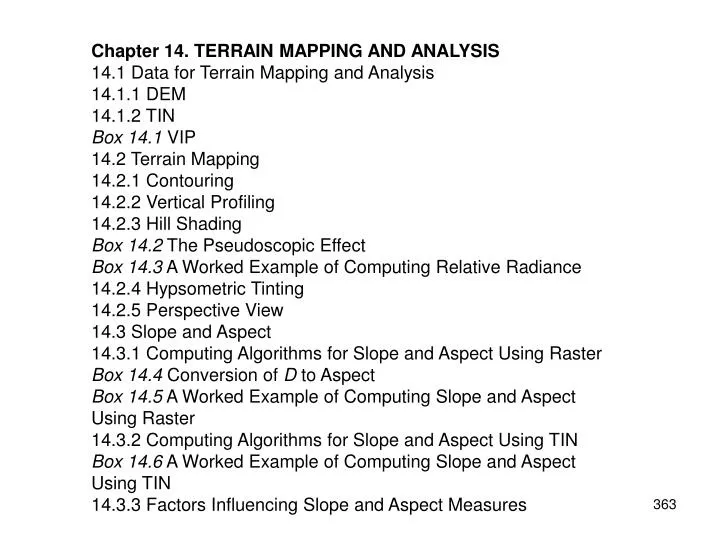
Chapter 14. TERRAIN MAPPING AND ANALYSIS 14.1 Data for Terrain Mapping and Analysis 14.1.1 DEM

Chapter 14. TERRAIN MAPPING AND ANALYSIS 14.1 Data for Terrain Mapping and Analysis 14.1.1 DEM 14.1.2 TIN Box 14.1 VIP 14.2 Terrain Mapping 14.2.1 Contouring 14.2.2 Vertical Profiling 14.2.3 Hill Shading Box 14.2 The Pseudoscopic Effect Box 14.3 A Worked Example of Computing Relative Radiance 14.2.4 Hypsometric Tinting 14.2.5 Perspective View 14.3 Slope and Aspect 14.3.1 Computing Algorithms for Slope and Aspect Using Raster Box 14.4 Conversion of D to Aspect Box 14.5 A Worked Example of Computing Slope and Aspect Using Raster 14.3.2 Computing Algorithms for Slope and Aspect Using TIN Box 14.6 A Worked Example of Computing Slope and Aspect Using TIN 14.3.3 Factors Influencing Slope and Aspect Measures

14.4 Surface Curvature Box 14.7 A Worked Example of Computing Surface Curvature 14.5 Raster Versus TIN Box 14.8 Terrain Mapping and Analysis Using ArcGIS Key Concepts and Terms Review Questions Applications: Terrain Mapping and Analysis Task 1: Use DEM for Terrain Mapping Task 2: Derive Slope, Aspect, and Curvature from DEM Task 3: Build and Display a TIN Challenge Question References

Data for Terrain Mapping and Analysis • DEM (digital elevation model) and TIN (triangulated irregular network) are two common types of input data for terrain mapping and analysis. • A DEM represents a regular array of elevation points. It can be converted to an elevation raster by placing each elevation point at the center of a cell. • A TIN approximates the land surface with a series of nonoverlapping triangles. • A DEM can be converted into a TIN by using the maximum z-tolerance algorithm or the VIP (very important point) algorithm. • A TIN can be converted into a DEM by using local first-order polynomial interpolation.

Figure 14.1 Peis the estimated elevation, Phis the actual elevation, and d is the offset between Peand Ph at cell P. VIP uses s, a distance between Ph and the hypothetical surface between G and C, for measuring the significance of P.

Input Data to TIN Besides DEM, a TIN can also use additional point data such as surveyed elevation points, GPS (global positioning system) data, and LIDAR data; line data such as contour lines and breaklines; and area data such as lakes and reservoirs.

Figure 14.2 A breakline, shown as a dashed line in (b), subdivides the triangles in (a) into a series of smaller triangles in (c).

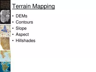
Terrain Mapping Terrain mapping techniques include contouring, vertical profiling, hill shading, hypsometric tinting, and perspective view.

Figure 14.3 A contour line map.

Figure 14.4 The contour line of 900 connects points that are interpolated to have the value of 900 along the triangle edges.

Figure 14.5 A vertical profile.

Figure 14.6 An example of hill shading, with the sun’s azimuth at 315° (NW) and the sun’s altitude at 45°.

Figure 14.7 A hypsometric map. Different elevation zones are shown in different gray symbols.

Figure 14.8 A 3-D perspective view.

Figure 14.9 Three controlling parameters of the appearance of a 3-D view: the viewing azimuth a is measured clockwise from the north, the viewing angle u is measured from the horizon, and the viewing distance d is measured between the observation point and the 3-D surface.

Figure 14.10 Draping of streams and shorelines on a 3-D surface.

Figure 14.11 A 3-D perspective view of an elevation zone map.

Figure 14.12 A view of 3-D buildings in Boston, Massachusetts.

Slope and Aspect • Slopemeasures the rate of change of elevation at a surface location. Slope may be expressed as percent slope or degree slope. • Aspect is the directional measure of slope. Aspect starts with 0° at the north, moves clockwise, and ends with 360° also at the north. Because it is a circular measure, We often have to manipulate aspect measures before using them in data analysis.

Figure 14.13 Slope, either measured in percent or degrees, can be calculated from the vertical distance a and the horizontal distance b.

Figure 14.14 Aspect measures are often grouped into the four principal directions (top) or eight principal directions (bottom).

Figure 14.15 Transformation methods to capture the N–S direction (a), the NE–SW direction (b), the E–W direction (c), and the NW–SE direction (d).

Computing Algorithms for Slope and Aspect Using Raster • The slope and aspect for an area unit (i.e., a cell or triangle) are measured by the quantity and direction of tilt of the unit’s normal vector—a directed line perpendicular to the unit. • Different approximation (finite difference) methods have been proposed for calculating slope and aspect from an elevation raster. Usually based on a 3-by-3 moving window, these methods differ in the number of neighboring cells used in the estimation and the weight applying to each cell.

Figure 14.16 The normal vector to the cell is the directed line perpendicular to the cell. The quantity and direction of tilt of the normal vector determine the slope and aspect of the cell. (Redrawn from Hodgson, 1998, CaGIS 25, (3): pp. 173–185; reprinted with the permission of the American Congress on Surveying and Mapping.)

Figure 14.17 Ritter’s algorithm for computing slope and aspect at C0 uses the four immediate neighbors of C0.

Figure 14.18 Horn’s algorithm for computing slope and aspect at C0 uses the eight neighboring cells of C0. The algorithm also applies a weight of 2 to e2, e4, e5, and e7, and a weight of 1 to e1, e3, e6, and e8.

Computing Algorithms for Slope and Aspect using TIN The x, y, and z values of points that make up a TIN are used to compute slope and aspect for each triangle.

Figure 14.19 The algorithm for computing slope and aspect of a triangle in a TIN uses the x, y, and z values at the three nodes of the triangle.

Factors Influencing Slope and Aspect Measures Factors that can influence slope and aspect measures include the resolution of DEM, the quality of DEM, the computing algorithm, and local topography.

Figure 14.20 DEMs at three different resolutions: USGS 30-meter DEM (a), USGS 10-meter DEM (b), and 1.83-meter DEM derived from LIDAR data (c).

Figure 14.21 Slope layers derived from the three DEMs in Figure 14.19. The darkness of the symbol increases as the slope becomes steeper.

Surface Curvature Surface curvature measures can determine if the surface at a cell location is upwardly convex or concave.

National Elevation Dataset http://gisdata.usgs.gov/ned/

Chapter 14. TERRAIN MAPPING AND ANALYSIS 14.1 Data for Terrain Mapping and Analysis 14.1.1 DEM