Download
1 / 37
390 likes | 912 Views
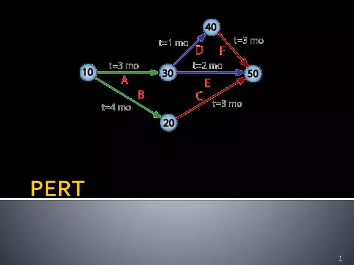
PERT. The Program (or Project ) Evaluation and Review Technique , commonly abbreviated PERT ,

E N D
The Program (or Project) Evaluation and Review Technique, commonly abbreviated PERT, • is a model for project management designed to analyze and represent the tasks involved in completing a given project. It is commonly used in conjunction with the critical path method or CPM.
A Gantt chart created using Microsoft Project (MSP). Note • the critical path is in red, • the slack is the black lines connected to non-critical activities, • since Saturday and Sunday are not work days and are thus excluded from the schedule, some bars on the Gantt chart are longer if they cut through a weekend.
Duration • Slack
Duration Calculate the duration
Optimistic time (O): • the minimum possible time required to accomplish a task, assuming everything proceeds better than is normally expected • Pessimistic time (P): • the maximum possible time required to accomplish a task, assuming everything goes wrong (but excluding major catastrophes). • Most likely time (M): • the best estimate of the time required to accomplish a task, assuming everything proceeds as normal.
Intuitively, we use a triangle distribution. max modal min
½*f(mo) *(ma-mi)=The area of the triangle=1 • f(mo)=2/(ma-mi) • 2/(ma-mi) mo ma mi
f(x1) / f(mo)=(x1-mi)/(mo-mi) • Similarly • 2/(ma-mi) • 2(ma-x2)/(ma-mo)/(ma-mi) • 2(x1-mi)/(mo-mi)/(ma-mi) • So • f(x){ • If(x>=mi&&x<=mo) return 2(x-mi)/(mo-mi)/(ma-mi); • if(x>=mo&&x<=ma) return 2(ma-x)/(ma-mo)/(ma-mi); • else{return 0;} • } x1 x2 ma mo mi
The expectation will be • =(min + modal + max) / 3; • variance() { • return • (min * min + modal * modal + max * max - min * modal - modal * max - max * min) / 18; • }
Triangle is not smooth. • The density changes too ACUTELY, esp. around the modal. • So we’ll try a smooth one • norm distribution?
spans out of the range(mi,ma)? • Truncate • If at 3sigma, then • sigma=(ma-mi)/6 • Modal • Need to be twisted. • Beta distribution comes into our attention.
Beta Distribution Where For a=0,b=1
Get the alpha and beta such that • Shape Like Normal Distribution • Kurtosis • A high kurtosis distribution has a sharper peak and longer, fatter tails, while a low kurtosis distribution has a more rounded peak and shorter thinner tails. • Normal Distribution is mesokurtic • With the same var • as Normal Distribution truncated at (-3sigma,3sigma)
Such a BetaDist • a=1+4(mo-mi)/(ma-mi) • b=1+4(ma-mo)/(ma-mi) • TE = (O + 4M + P) ÷ 6 • sVar =(ma-mi)/6
Expected time (TE): • the best estimate of the time required to accomplish a task, assuming everything proceeds as normal • (the implication being that the expected time is the average time the task would require if the task were repeated on a number of occasions over an extended period of time).
ES & EF • The first step is to determine the ES and EF. • The ES is defined as the maximum EF of all predecessor activities, unless the activity in question is the first activity, for which the ES is zero (0). • The EF is the ES plus the task duration (EF = ES + duration).
The ES for start is zero since it is the first activity. Since the duration is zero, the EF is also zero. This EF is used as the ES for a and b. • The ES for a is zero. The duration (4 work days) is added to the ES to get an EF of four. This EF is used as the ES for c and d. • The ES for b is zero. The duration (5.33 work days) is added to the ES to get an EF of 5.33. • The ES for c is four. The duration (5.17 work days) is added to the ES to get an EF of 9.17. • The ES for d is four. The duration (6.33 work days) is added to the ES to get an EF of 10.33. This EF is used as the ES for f. • The ES for e is the greatest EF of its predecessor activities (b and c). Since b has an EF of 5.33 and c has an EF of 9.17, the ES of e is 9.17. The duration (5.17 work days) is added to the ES to get an EF of 14.34. This EF is used as the ES for g. • The ES for f is 10.33. The duration (4.5 work days) is added to the ES to get an EF of 14.83. • The ES for g is 14.34. The duration (5.17 work days) is added to the ES to get an EF of 19.51. • The ES for finish is the greatest EF of its predecessor activities (f and g). Since f has an EF of 14.83 and g has an EF of 19.51, the ES of finish is 19.51. Finish is a milestone (and therefore has a duration of zero), so the EF is also 19.51.
LS &LF • The next step is to determine the late start (LS) and late finish (LF) of each activity. • This will eventually show if there are activities that have slack. • The LS is the LF minus the task duration (LS = LF - duration).
The LF for finish is equal to the EF (19.51 work days) since it is the last activity in the project. Since the duration is zero, the LS is also 19.51 work days. This will be used as the LF for f and g. • The LF for g is 19.51 work days. The duration (5.17 work days) is subtracted from the LF to get an LS of 14.34 work days. This will be used as the LF for e. • The LF for f is 19.51 work days. The duration (4.5 work days) is subtracted from the LF to get an LS of 15.01 work days. This will be used as the LF for d. • The LF for e is 14.34 work days. The duration (5.17 work days) is subtracted from the LF to get an LS of 9.17 work days. This will be used as the LF for b and c. • The LF for d is 15.01 work days. The duration (6.33 work days) is subtracted from the LF to get an LS of 8.68 work days. • The LF for c is 9.17 work days. The duration (5.17 work days) is subtracted from the LF to get an LS of 4 work days. • The LF for b is 9.17 work days. The duration (5.33 work days) is subtracted from the LF to get an LS of 3.84 work days. • The LF for a is the minimum LS of its successor activities. Since c has an LS of 4 work days and d has an LS of 8.68 work days, the LF for a is 4 work days. The duration (4 work days) is subtracted from the LF to get an LS of 0 work days. • The LF for start is the minimum LS of its successor activities. Since a has an LS of 0 work days and b has an LS of 3.84 work days, the LS is 0 work days.
Slack • Float or Slack • is the amount of time that a task in a project network can be delayed without causing a delay
Slack • Slack is computed in one of two ways, slack = LF - EF or slack = LS - ES. Activities that are on the critical path have a slack of zero (0). • The duration of path adf is 14.83 work days. • The duration of path aceg is 19.51 work days. • The duration of path beg is 15.67 work days.
Slack • Start and finish are milestones and by definition have no duration, therefore they can have no slack (0 work days). • The activities on the critical path by definition have a slack of zero; however, it is always a good idea to check the math anyway when drawing by hand. • LFa - EFa = 4 - 4 = 0 • LFc - EFc = 9.17 - 9.17 = 0 • LFe - EFe = 14.34 - 14.34 = 0 • LFg - EFg = 19.51 - 19.51 = 0 • Activity b has an LF of 9.17 and an EF of 5.33, so the slack is 3.84 work days. • Activity d has an LF of 15.01 and an EF of 10.33, so the slack is 4.68 work days. • Activity f has an LF of 19.51 and an EF of 14.83, so the slack is 4.68 work days. • Therefore, activity b can be delayed almost 4 work days without delaying the project. Likewise, activity dor activity f can be delayed 4.68 work days without delaying the project (alternatively, d and f can be delayed 2.34 work days each).
CP • The critical path is aceg and the critical time is 19.51 work days. • It is important to note that there can be more than one critical path (in a project more complex than this example) • or that the critical path can change. • For example, let's say that activities d and f take their pessimistic (b) times to complete instead of their expected (TE) times. The critical path is now adf and the critical time is 22 work days. On the other hand, if activity c can be reduced to one work day, the path time for aceg is reduced to 15.34 work days, which is slightly less than the time of the new critical path, beg (15.67 work days).
MS Project • Project中的PERT分析技术 • 在Project中可以执行“计划评审技术”(PERT)来评估任务工期。在为任务指定了乐观工期、悲观工期和预期工期之后,Project 就会自动计算这3个工期的加权平均值。在默认情况下,PERT 分析中的权数是按照1:4:1分配给乐观工期、最可能工期和悲观工期的。当然,用户也可根据实际情况调整这3个权数。 • Project为PERT分析专门制作了工具栏,下图为“PERT工具栏”
【例6-5】修改PERT权数 • (1)打开PERT工具栏:选择菜单【视图】/【工具栏】/【PERT分析】,系统启动如上图所示的PERT分析工具栏。 • (2)单击“设置PERT权重”按钮,弹出如下所示对话框。
3.乐观、悲观和预期甘特图 • 既然每项任务都存在乐观、悲观和预期工期,对应地,根据这些数据可以分别计算项目与任务的时间参数,也就有了乐观、悲观和预期甘特图,它们都是甘特图的变体。 • 这3个变化后的甘特图,只有在使用 PERT 分析工具后才可用,而使用PERT 分析工又以加载PERT分析“组件对象模型”(COM) 加载项为前提。 • “预期甘特图”视图——与 PERT 分析结合使用,有助于估算任务的预期工期、开始日期和完成日期。 使用“预期甘特图”视图可以进行如下操作: • 输入项目任务的预计工期。 • 比较任务工期估计值之间的差别。 • “预期甘特图”视图的默认工作列表是“预期状况”表。
PERT 项工作表 • “PERT项工作表”的作用是帮助用户估算任务的确切工期。用户可以在该表重输入任务的乐观、预期和悲观工期,然后让 Project 计算最终的工期值t。通过更改 Project 赋予3个估计工期的权重,可以调整工期的估计值使其更加精确。 • “PERT 项工作表”视图是“任务工作表”视图的一个变体。只有在加载了PERT分析“组件对象模型”(COM) 加载项后方能使用。“PERT 项工作表”视图操作的默认表是“PERT 项”表。 • 【例6-6】使用PERT分析估计任务工期 • 项目“06-06-begin.mpp”如下图,此时只有任务列表,工期、链接关系尚未设定。请按照如下步骤进行操作,使用PERT方法分析任务工期,结果保存为“06-06-over.mpp”。
【分析】完成该工作,需要使用到Project所提供的PERT分析功能,在使用PERT分析前,必须先加载“组件对象模型COM加载宏”。【分析】完成该工作,需要使用到Project所提供的PERT分析功能,在使用PERT分析前,必须先加载“组件对象模型COM加载宏”。 • (1)首先加载COM加载宏;选择菜单【工具】/【自定义】/【工具栏】,弹出“自定义”对话框,如下图所示。选择“命令”页,在左边“类别”栏中选择“工具”,在右边“命令”列表中选择“COM加载项”。 • (2)在上述对话框中,单击右侧列表中的“COM加载项”这一项,按住鼠标左键不放,将该项拖到工具栏中适当位置再释放(位置决定于用户的习惯),该命令将显示在指定位置。 • 加载完毕后就可以进行项目的PERT分析计算了。 • (3)单击工具栏中刚放入的按钮,弹出如下对话框,保证“PERT分析”前的复选框打勾,再单击确定按钮。