Download
1 / 30
300 likes | 386 Views
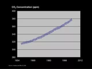
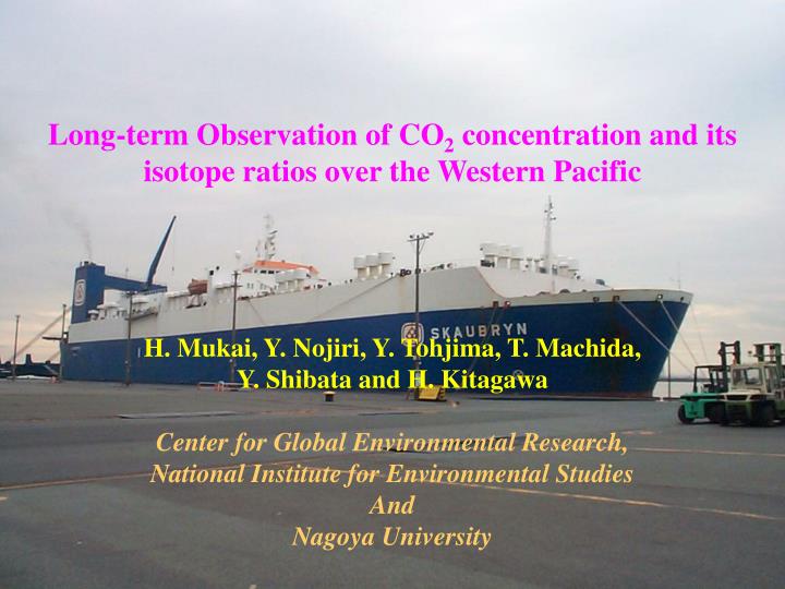
Long-term Observation of CO 2 concentration and its isotope ratios over the Western Pacific. H. Mukai, Y. Nojiri, Y. Tohjima, T. Machida, Y. Shibata and H. Kitagawa Center for Global Environmental Research, National Institute for Environmental Studies And Nagoya University.

E N D
Long-term Observation of CO2 concentration and its isotope ratios over the Western Pacific H. Mukai, Y. Nojiri, Y. Tohjima, T. Machida, Y. Shibata and H. Kitagawa Center for Global Environmental Research, National Institute for Environmental Studies And Nagoya University
Monitoring by using commercial cargo ships AtmosphericCO2 samples from wide range of latitude can be colleted. Frequent commercial cargo ship service enable us to observed seasonal variation of CO2 in addition to long-term variation. Japan-Oceania cruise can provide us a good chance to observe latitudinal difference in behavior of CO2 from Northern Hemisphere to Southern Hemisphere. Relatively economic monitoring if it goes as planed.
MOLGlory Alligator Hope(MOL) 92 93 94 95 96 97 98 99 00 01 02 03 04 05 06 07 SKAUBRYN(Seaboard) NOV Japan - N America (30N-55N) SKAUGRAN(Seaboard) PYXIS(TOYOFUJI) Japan – Oceania (30N-35S) Southern Cross Hakuba FUJITRANS WORLD Golden Wattle(MOL) Trans Future Special thanks to MOL, Toyofuji, Fuji Trans, Nihhon Usen, Seaboard International Shipping Co.
FUJITRANS WORD and PYXIS routes 2003 Sep – 2004 Nov PYXIS FUJITRANS WORLD
Bottle Sampling : • Stainless-steel bottle 3L (+ Glass bottle 2.5L ) • ~10 times/y since 1995 • ~ 3 samples / 10 degree in latitude • 2) Gas analysis in the bottle: • CO2, N2O, CH4 (NDIR, GC-ECD, GC-FID) • delta 13C, delta 18O (MAT252, dual inlet) • 14C is measured by Accelerator MASS in NIES
GPS sensor Temperature sensor Air Inlet
Sampling Controller GPS receiver CO2 analyzer (3) Sampling Flask Box (2) Cooler (-45 oC) (1) Metal bellows pump
Isotope signature of CO2 (13C, 14C, 18O) will provide important clues about CO2 budget and climatic effects on CO2 uptake mechanism 14CO2 12CO2 13CO2 C3 plant 12C18O2 H218O C4 plant Soil
40N-50N 20N-30N CO2 Delta 13C Delta 18O 0-10N 20S-10S
CO2 concentration Delta 13C Latitudinal distribution
CO2 growth rate (ppm/y) Delta 13C change rate (per mil/y)
Biological Discrimination Simple Global Flux Estimation 12C flux dCa/dt = CF + CNs + CNb------------------(1) 13C flux dδ13Ca/dt = CFδF+ CNs(δa +εas) + CNb(δa +εab) + CGs(δs –δa) + CGb(δb –δa) ------(2) CF = anthropegenic input ( Fossil combustion and Cement production) CNs = Net Sea flux CNb = Net land biological flux CGS = Gross exchange flux between Sea and atmosphere CGb = Gross exchange flux between land biosphere and atmosphere Isotope disequilibrium term CGs(δs –δa) + CGb(δb –δa) = 93 Gt-C per mli / year (Francey et al )
Preliminary estimation of flux Anthropogenic input Atmosphere Land Biosphere Ocean
15S 25N
A preliminary guess of net Carbon flux budget (PgC/y) to assess isotope signature and its usability These values for terrestrial and oceanic sinks may have a large uncertainty (over +1Pg/y)
Assessment of isotopic balance equation Oceanic sink looked too variable. Oceanic sink variation = +1 PgC and decrease trend ??? c.f. Reported oceanic variation on flux is about +0.4 PgC What is possible causes ? If we set Oceanic sink variation to be Zero How much percent we have to change the parameters such as Discrimination factor? It is most important for both disequilibrium and biological uptake term. 1) Discrimination for CO2 uptake by plants fractionation factor decreases? C4 plant fraction to C3 plant increase? 2) Gross primary production decreases or increase?
Apparent variation of oceanic sink can be compensated by biological discrimination adjustment by up to 0.2 per mil SOI 0.2 per mil decrease can be possible by high T and low humidity , but Gross primary production can not decrease by corresponding amount (over 50%)
El Nino Delta 18O trend showed some increase over 10 years SOI Increase delta 18O of water? GPP decrease?
Conclusion • Ten-year observation of CO2 and isotopes over Western Pacific from 30S to 50N was conducted by using 8 commercial cargo ships. • (2) By simple carbon budget equations using isotopic data, oceanic and terrestrial uptake amounts were estimated. Oceanic sink was relatively stable but still had 1Pg-C variation. Terrestrial sink seemed to decrease rapidly by higher and more dry condition at El Nino event. Apparent oceanic fluctuation may be partly caused by the change of C isotopic discrimination due to climatic condition. • (3) Oxygen isotope ratio showed increasing trends in all latitude during 10 years. • It was different tendency from that of 1990’s. It may be related to high temperature and low humidity tendency including lower GPP in recent years. • (4) Carbon-14 measurements will give an another angle to look at carbon budget. Further analysis is needed. • (5) Seasonal variations of CO2 and carbon isotope ratio were large in Northern Hemisphere but small in Southern Hemisphere. Isotope fractionation factor was about –19 per mil on average, but –14 per mil in 20S, which showed some C4 plants effect at that latitude. (not shown)
Seasonal component and biological discrimination Apparent Biological discrimination -19 per mil Source and sink delta 13C
CF: Merland δF: -28 per mil (estimated) εas: 1.8 per mil εab: 19 per mil Gb: 125PgC/y Go: 90PgC/y Disequilibrium Sea-Atmosphere: 0.6 per mil Disequilibrium Terrestrial biosphere-Atmosphere: 0.394 as standard case
Oxygen isotope ratio delta 18O