Download
1 / 54
540 likes | 758 Views
Chapter 9. Risk And Capital Budgeting. Dr. Del Hawley FIN 634 Fall 2003. Choosing the Right Discount Rate. What discount rate should managers use in capital budgeting? Rate should reflect the opportunity cost of all of the firm’s investors (the cost of capital)

E N D
Chapter 9 Risk And Capital Budgeting Dr. Del HawleyFIN 634Fall 2003
Choosing the Right Discount Rate • What discount rate should managers use in capital budgeting? • Rate should reflect the opportunity cost of all of the firm’s investors (the cost of capital) • Rate should also reflect the risk of the specific project • To find discount rate, start with simplifying assumptions: • Assume all equity financing, so only have to satisfy S/Hs • Assume firm makes all investments in a single industry • These allow firm to use the cost of equity as discount rate • Know from MBA 611 that the cost of equity is found with the CAPM (Eq 9.1)
Determining All Leather’s Cost of Equity • All Leather, Inc., an all-equity firm that produces leather sofas, is evaluating a proposal to build a new manufacturing facility. • As a producer of luxury goods, the firm’s performance is very sensitive to economic conditions. This is reflected in the firm’s 1.3 stock beta. • Note: The higher risk must be reflected in the discount rate used to evaluate the new manufacturing facility unless the project’s risk is not average relative to the firm’s other current investments.
Determining All Leather’s Cost of Equity • Based on current market conditions, the financial manager will use Rf = 4%. Her market analysis provided an expected market return of 9%. • Can use CAPM to find All Leather’s cost of equity: E(Re ) = Rf + (E(Rm) - Rf) = 4% + 1.3 (9% - 4%) =10.5% cost of equity
How to Choose Rf in the CAPM E(Re ) = Rf + (E(Rm) - Rf) Any rate on the yield curve for government securities is a risk-free rate. So which one do you use? • Today’s yield curve runs from about 1.5% to 5% on risk-free yields. This is wide spread by historical standards. • Since you will be using the CAPM to set a discount rate for long-term investments, you need the market’s estimate of the inflation premium, but you do not need the other parts of the long-term rate that have to do with liquidity or preferences.
How to Choose Rf in the CAPM The Adjusted T-Bond Method uses the current rate on a 20-year T-Bond less the average spread between 20-year and 1-year T-bonds – about 1.2% Current yield on 20-year T-Bond 5.0% Less the average spread -1.2% Adjusted T-Bond Rate 3.8% Current Yield on a 1-year T-Bill 1.5%
How to Choose RM in the CAPM RM needs to be the expected rate of return on the market portfolio in the future, on average, over a long time. How do we know that?
How to Choose RM in the CAPM RM needs to be the expected rate of return on the market portfolio in the future, on average, over a long time. How do we know that? Base it on recent market performance?
How to Choose RM in the CAPM RM needs to be the expected rate of return on the market portfolio in the future, on average, over a long time. How do we know that? Base it on recent market performance? No. Recent past performance is a very poor predictor of long-term future performance. (See the link on our website for annual stock returns.)
How to Choose RM in the CAPM RM needs to be the expected rate of return on the market portfolio in the future, on average, over a long time. How do we know that? Base it on past long-term performance? The average annual return on the market over the last 74 years is about 11.6%.
How to Choose RM in the CAPM RM needs to be the expected rate of return on the market portfolio in the future, on average, over a long time. How do we know that? Base it on past long-term performance? The average annual return on the market over the last 74 years is about 11.6%. If you always use 11.6% as RM, you lock the SML to that point so it decreases slope as Rf rises and increases slope as Rf falls. This is just about opposite of what you would expect to happen.
How to Choose RM in the CAPM RM needs to be the expected rate of return on the market portfolio in the future, on average, over a long time. How do we know that? Base it on market risk premium? On average over a long time, this has been about 5.6%.
How to Choose RM in the CAPM RM needs to the expected rate of return on the market portfolio in the future, on average, over a long time. How do we know that? Base it on market risk premium? On average over a long time, this has been about 5.6%. This method has the best economic basis for what we are doing, and it is very simple. Using this method, the CAPM is used simply as: E(Re ) = Adjusted Rf + ( 5.6% )
Finding All Leather’s Cost of Equity (Cont) • Other operating factors impact beta: • Cost structure and production process • Mix of variable and fixed costs • Volatility of operating cash flow (EBIT) will rise with fixed operating costs • Substituting fixed for variable costs increases profits more than proportionally when sales increase, but hurts more if sales fall
Finding All Leather’s Cost of Equity (Cont) Define degree of operating leverage (DOL) as the expected % in EBIT divided by the expected % in sales. Estimate DOL as DOL = (Sales – Total VC)/EBIT = Total Contribution Margin / EBIT High DOL: small change in sales large change in EBIT • Note key terms: EBIT= contribution margin - fixed costs • Contribution margin = gross profit per unit of sales • Gross profit = price per unit - variable cost per unit (Eq 9.2)
Financial Data for All Leather Inc. and Microfiber Corp. All Leather’s additional operating leverage results in a larger percentage change in EBIT for a change in sales than Microfiber. - Larger volatility of cash flows to support debt - Larger volatility of cash flows to shareholders
Operating Leverage for All Leather and Microfiber EBIT All Leather Microfiber Sales
Impact of Operating Leverageon Costs of Debt and Equity • QUESTION: Does an increase in operating leverage result in an increase in the cost of debt, other things equal?
Impact of Operating Leverageon Costs of Debt and Equity • QUESTION: Does an increase in operating leverage result in an increase in the cost of debt, other things equal? • YES (in general) because it increases the volatility of cash flows that are needed to pay the interest payments on the debt.
Impact of Operating Leverageon Costs of Debt and Equity • QUESTION: Does an increase in operating leverage result in an increase in the cost of debt, other things equal? • YES (in general) because it increases the volatility of cash flows that are needed to pay the interest payments on the debt. • QUESTION: Does an increase in operating leverage result in an increase in the cost of equity, other things equal?
Impact of Operating Leverageon Costs of Debt and Equity • QUESTION: Does an increase in operating leverage result in an increase in the cost of debt, other things equal? • YES (in general) because it increases the volatility of cash flows that are needed to pay the interest payments on the debt. • QUESTION: Does an increase in operating leverage result in an increase in the cost of equity, other things equal? • IT DEPENDS on how closely variations in sales are linked to changes in general economic conditions. In other words, it depends of whether the sales volatility is due to systematic or unsystematic risk.
Measuring Financial Leverage and its Impact on Firm’s Stock Beta • Firms also use fixed cost financing (debt and preferred stock) to magnify the effect of a given change in EBIT on net income. This is called financial leverage. • Measured as the degree of financial leverage (DFL) • Estimate DFL as DFL = EBIT / EBT • Financial leverage can increase expected net profits, but it also increases risk • Thus, an increase in financial leverage can also increase a firm’s stock beta, and therefore its cost of equity.
Measuring Financial Leverage and its Impact on Firm’s Stock Beta
Measuring Financial Leverage and its Impact on Firm’s Stock Beta
The Weighted Average Cost of Capital (WACC) For firm’s that have both equity and debt in the capital structure, use the weighted avg cost of capital (WACC) as the discount rate. Demonstrate using Comfy Inc’s capital structure: • Comfy Inc builds residential houses • Firm has $150mn equity (E), with cost of equity re= 12.5% • Also has bonds (D) outstanding worth $50mn, with rd = 6.5% Calculate WACC = 11% as follows:
Finding the WACC (Cont) How can Comfy’s managers be sure WACC = 11%? • First way: assume wealthy investor purchases all firm’s debt and equity. This is the return he/she would earn. • Second way: Suppose the firm invests in a project earning 11% and distributes its return to the investors. Will they be satisfied? The following table shows that the cash flows generated and distributed satisfy the investors’ claims:
Finding WACC for Firms with Complex Capital Structures How do you estimate the WACC if a firm has long-term (LT) debt as well as preferred (P) and common stock (E)? Find weighted average of the individual capital costs:
Finding WACC for Firms with Complex Capital Structures Assume S.N. Sherwin Co. wants to determine its WACC • Has 10,000,000 common shares O/S; price = $15/sh; rc = 15% • Has $40mn L-T, fixed rate notes with 8% coupon rate, but 7% YTM; notes sell at premium and worth $49mn • Has 500,000 pref shrs, $2 annual dividend, $25 price, $12.5mn value Total value = $150m E+ $49m LT+$12.5m P = $211.5m
Connecting the WACC to the CAPM Although they were developed separately, WACC is consistent with the CAPM. In fact, you can use the CAPM to estimate the cost of any security. • To calculate the beta for bonds of a large corporation: • First find covariance between the bonds and the stock market, then • Plug computed debt beta (d),Rf & Rm into CAPM to find rd • The debt beta is typically quite low for healthy, low-debt firms • The debt beta rises with leverage, and approaches the equity beta in high-debt companies. If Comfy’s debt beta is 0.1, then the CAPM estimate of its cost of debt is:
Calculating Asset Betas and Equity Betas • The CAPM establishes a direct link between the required return and the betas of securities. • The firms ASSET Beta equals the weighted average of the debt and equity betas: (Eq 9.4) • A firm’s asset beta thus equals the covariance of the firm’s CFs with RM, divided the variance the market’s return. • For an all-equity firm, the asset beta = equity beta • For a levered firm, the asset beta will be less than equity beta • If the asset beta is known and the debt beta is assumed to be 0, the equity beta can be computed directly from A (Eq 9.5)
Finding Equity Betas from Asset Betas, and Vice Versa (Cont) • Can only use Eq 9.5 if debt beta assumed = 0 • Since debt = 20% of capital and equity = 80%, the debt-to-equity ratio D/E = 0.2 ÷ 0.8 = 0.25 • Not surprisingly, equity beta is higher if debt beta assumed 0
Finding Equity Betas from Asset Betas, and Vice Versa (Cont) • Can now state decision rule for determining the discount rate to use for projects with asset betas similar to the firm’s own: • For an all equity firm, use the cost of equity given by the CAPM • For a levered firm, use the WACC computed using the CAPM and the betas of the individual capital components • If a project’s asset beta differs from firm’s asset beta, must compute and use project betas.
Finding the Discount Rate to Use for Projects Unrelated to Firm’s Industry What if a company has diversified investments in many industries? • In this case, using the firm’s WACC to evaluate an individual project would be inappropriate. Instead, use the project’s asset beta adjusted for desired leverage.
Finding the Discount Rate to Use for Projects Unrelated to Firm’s Industry Assume GE is evaluating an investment in the oil & gas industry. This is much different from any of GE’s existing businesses. • GE should examine existing firms that are pure plays (public firms operating only in the O&G industry). Say GE selects Berry Petroleum and Forest Oil as pure plays: • They are operationally similar firms, but Berry Petroleum’s E = 0.65 and Forest Oil’s E = 0.90. Why so different? • Forest uses debt for 39% of its financing, while Berry has only 14% debt in its capital structure. Even if the core businesses have the same risk (A equal), E will differ because of the differences in financial leverage.
Data for Berry Petroleum and Forest Oil • Computed using Eq 9.4 and assuming debt beta = 0 • Berry Petrol: A = (%D)d + (%E)E = (0.14)(0) + (0.86)(0.65) = 0.56 • Forest Oil: A = (%D)d + (%E)E = (0.39)(0) + (0.61)(0.90) = 0.55
Converting Equity Betas to Asset Betas for Two Pure Play Firms • To determine the correct A to use as discount rate for GE’s O&G project, convert the pure play E to the A, then average. • The previous table lists the data needed to compute the unlevered equity beta for each of the surrogates. • The unlevered equity beta (same as A) strips out the effect of financial leverage, so it’s always less than or equal to the equity beta for a company. • Berry’s A = 0.56, Forest’s A = 0.55, so average A = 0.55 • GE’s capital structure consists of 20% debt and 80% equity (D/E ratio = 0.25). So, compute the relevered equity beta for GE as follows:
Converting Equity Betas to Asset Betas for Two Pure Play Firms (Continued) • Now assume that the risk-free rate of interest is 6% and the expected risk premium on the market is 7% • Using the CAPM equation, compute the rate of return GE shareholders require for the oil and gas investment: E(R) = 6% + 0.69(7%) = 10.83% • The final step to find the right discount rate for GE’s investment in this industry is to calculate the project’s WACC: • GE’s financing is 80% equity and 20% debt. Assume investors expect 6.5% on GE’s bonds
Summarizing Rules for Selecting an Appropriate Project Discount Rate • When an all equity firm invests in an asset similar to its existing assets, the cost of equity is the appropriate discount rate to use in NPV calculations. • When a levered firm invests in an asset similar to its existing assets, the WACC is the right discount rate. • When a firm invests in an asset that is different than its existing assets, it should look for pure play firms to find the right discount rate. • Firms can calculate an industry asset beta by unlevering the betas of pure play firms • Given the industry asset beta, firms can determine an appropriate discount rate using the CAPM
Accounting for Taxes in Finding WACC • We have thus far assumed away taxes, but taxes (or the exclusion of taxes on interest payments0 are ften important. • Tax deductibility of interest payments favors use of debt • Accounting for interest tax shields yields the after-tax WACC (Eq 9.6) • From Eq. 9.6, we can likewise present a method for computing the after-tax equity beta from the asset beta. Again assuming debt beta = 0, the equity beta is given by: (Eq 9.7)
A Closer Look at RiskBreak-Even Analysis A key component in assessing operating risk is finding the break-even point (BEP). • BEP is the level of output (units of product sold) where all operating costs (fixed and variable) are covered. • BEP is found by dividing Fixed Operating Costs (FC) by the the contribution margin per unit (CM)
A Closer Look at RiskBreak-Even Analysis Use this to find the BEP for All Leather and Microfiber • All Leather: FC = $10,000,000; Pr = $950/un; VC = $600/unit • Microfiber: FC = $2,000,000; Pr = $950/un; VC = $800/unit
Break-Even Point for All Leather Costs & Revenues Total revenue Total costs $10,000,000 Fixed costs 28,572 units Units All Leather has high fixed costs ($10,000,000), but also high contribution margin ($350/sofa). High BEP, but once FC covered, profits grow rapidly.
Break-Even Point for Microfiber Costs & Revenues Total revenue Total costs Fixed costs $2,000,000 13,334 units Units Microfiber has low fixed costs ($2,000,000), but also low contribution margin ($150/sofa). Low BEP, but profits grow slowly after FC covered.
Sensitivity Analysis Sensitivity analysis allows mangers to test the importance of each assumption underlying a forecast. Best Electronics Inc (BEI) has a new DVD player project. Base case assumptions (below) yield E(NPV) = $1,139,715 • 1. The project’s life is five years. • 2. The project requires an up-front investment of $41 million. • 3. BEI will depreciate initial investment on S-L basis for five years • 4. One year from now, DVD industry will sell 3,000,000 units • 5. Total industry unit volume will increase by 5% per year. • 6. BEI expects to capture 10% of the market in the first year • 7. BEI expects to increase its market share one percentage point each year after year one. • 8. The selling price will be $100 in year one. • 9. Selling price will decline by 5% per year after year one. • 10. Variable production costs will equal 60% of the selling price. • 11. The appropriate discount rate is 14 percent.
Sensitivity Analysis of DVD Project If all optimistic scenarios play out, project’s NPV rises to $37,635,010. If all pessimistic scenarios play out, project’s NPV falls to -$19,271,270!
Using Decision Trees to Make Multi-Step Investment Decisions • Many real investment projects are conditional & multi-stage: will only proceed to stage 2 if stage 1 successful • Occurs frequently with new product introductions • Begin selling in test market; if successful, build factory for full-scale production and nationwide roll-out • Very hard to evaluate in standard capital budgeting framework • Decision trees allow managers to break investment analysis into distinct phases • Forces managers to perform extended “if-then” analysis
Using Decision Trees to Make Multi-Step Investment Decisions Assume Trinkle Foods (Canada) has invented a new salt substitute, Odessa. Market testing will take place in Vancouver. • Market test will cost $5 million, but no new facilities are needed • If the test is successful, Trinkle will spend an additional $50mn to build a factory and launch nationwide one year later, after which Trinkle predicts $12mn NCF per year for 10 years • If the test is unsuccessful, Trinkle expects full product launch to generate only $2 mn NCF per year for 10 years. If Trinkle’s WACC=15% should Trinkle invest? If so, in what?
Using Decision Trees (Cont) • Next figure shows decision tree for investment problem • Initially, firm can choose to spend C$5 mn on market test • If market test executed, expect probability of success = 0.5 • Proper way to use tree: begin at end & work backwards • Suppose in one year, Trinkle learns test is successful. • At that point, the NPV of launching the product is: • Clearly, Trinkle would invest if it winds up on this branch