Download
1 / 93
930 likes | 937 Views
MapReduce Programming. MapReduce: Recap. Programmers must specify: map (k, v) → list(<k ’ , v ’ >) reduce (k ’ , list(v ’ )) → <k ’’ , v ’’ > All values with the same key are reduced together Optionally, also: partition (k ’ , number of partitions) → partition for k ’

E N D
MapReduce: Recap Programmers must specify: map (k, v) → list(<k’, v’>) reduce (k’, list(v’)) → <k’’, v’’> All values with the same key are reduced together Optionally, also: partition (k’, number of partitions) → partition for k’ Often a simple hash of the key, e.g., hash(k’) mod n Divides up key space for parallel reduce operations combine (k’, v’) → <k’, v’>* Mini-reducers that run in memory after the map phase Used as an optimization to reduce network traffic The execution framework handles everything else…
k1 v1 k2 v2 k3 v3 k4 v4 k5 v5 k6 v6 map map map map a 1 b 2 c 3 c 6 a 5 c 2 b 7 c 8 combine combine combine combine a 1 b 2 c 9 a 5 c 2 b 7 c 8 partition partition partition partition Shuffle and Sort: aggregate values by keys a 1 5 b 2 7 c 2 9 8 reduce reduce reduce r1 s1 r2 s2 r3 s3
“Everything Else” • The execution framework handles everything else… • Scheduling: assigns workers to map and reduce tasks • “Data distribution”: moves processes to data • Synchronization: gathers, sorts, and shuffles intermediate data • Errors and faults: detects worker failures and restarts • Limited control over data and execution flow • All algorithms must expressed in m, r, c, p • You don’t know: • Where mappers and reducers run • When a mapper or reducer begins or finishes • Which input a particular mapper is processing • Which intermediate key a particular reducer is processing
Tools for Synchronization • Cleverly-constructed data structures • Bring partial results together • Sort order of intermediate keys • Control order in which reducers process keys • Partitioner • Control which reducer processes which keys • Preserving state in mappers and reducers • Capture dependencies across multiple keys and values
Basic Hadoop API • Mapper • void map(K1 key, V1 value, OutputCollector<K2, V2> output, Reporter reporter) • void configure(JobConf job) • void close() throws IOException • Reducer/Combiner • void reduce(K2 key, Iterator<V2> values, OutputCollector<K3,V3> output, Reporter reporter) • void configure(JobConf job) • void close() throws IOException • Partitioner • void getPartition(K2 key, V2 value, int numPartitions) *Note: forthcoming API changes…
Data Types in Hadoop Writable Defines a de/serialization protocol. Every data type in Hadoop is a Writable. WritableComparable Defines a sort order. All keys must be of this type (but not values). Concrete classes for different data types. IntWritableLongWritable Text … Binary encoded of a sequence of key/value pairs SequenceFiles
Hadoop Map Reduce Example • See the word count example from Hadoop Tutorial
Word Count in Java publicclass MapClass extendsMapReduceBase implementsMapper<LongWritable, Text, Text, IntWritable> { privatefinalstaticIntWritable ONE = newIntWritable(1); publicvoid map(LongWritable key, Text value, OutputCollector<Text, IntWritable> out, Reporter reporter) throwsIOException { String line = value.toString(); StringTokenizer itr = newStringTokenizer(line); while(itr.hasMoreTokens()) { out.collect(newtext(itr.nextToken()), ONE); } } }
Word Count in Java publicclass ReduceClass extendsMapReduceBase implements Reducer<Text, IntWritable, Text, IntWritable> { publicvoidreduce(Text key, Iterator<IntWritable> values, OutputCollector<Text, IntWritable> out, Reporter reporter) throws IOException { int sum = 0; while(values.hasNext()) { sum += values.next().get(); } out.collect(key, new IntWritable(sum)); } }
Word Count in Java publicstaticvoid main(String[] args) throwsException { JobConf conf = newJobConf(WordCount.class); conf.setJobName("wordcount"); conf.setMapperClass(MapClass.class); conf.setCombinerClass(ReduceClass.class); conf.setReducerClass(ReduceClass.class); FileInputFormat.setInputPaths(conf, args[0]); FileOutputFormat.setOutputPath(conf, newPath(args[1])); conf.setOutputKeyClass(Text.class);// out keys are words (strings) conf.setOutputValueClass(IntWritable.class);// values are counts JobClient.runJob(conf); }
Word Count in Python with Hadoop Streaming Mapper.py: import sys for line in sys.stdin: for word in line.split(): print(word.lower() + "\t" + 1) Reducer.py: import sys counts = {} for line in sys.stdin: word, count = line.split("\t”) dict[word] = dict.get(word, 0) + int(count) for word, count in counts: print(word.lower() + "\t" + 1)
Basic Cluster Components • One of each: • Namenode (NN) • Jobtracker (JT) • Set of each per slave machine: • Tasktracker (TT) • Datanode (DN)
Putting everything together… namenode job submission node namenode daemon jobtracker tasktracker tasktracker tasktracker datanode daemon datanode daemon datanode daemon Linux file system Linux file system Linux file system … … … slave node slave node slave node
Anatomy of a Job • MapReduce program in Hadoop = Hadoop job • Jobs are divided into map and reduce tasks • An instance of running a task is called a task attempt • Multiple jobs can be composed into a workflow • Job submission process • Client (i.e., driver program) creates a job, configures it, and submits it to job tracker • JobClient computes input splits (on client end) • Job data (jar, configuration XML) are sent to JobTracker • JobTracker puts job data in shared location, enqueues tasks • TaskTrackers poll for tasks • Off to the races…
Mapper Mapper Mapper Mapper Mapper Intermediates Intermediates Intermediates Intermediates Intermediates Partitioner Partitioner Partitioner Partitioner Partitioner (combiners omitted here) Intermediates Intermediates Intermediates Reducer Reduce Reducer Source: redrawn from a slide by Cloduera, cc-licensed
Reducer Reduce Reducer RecordWriter RecordWriter RecordWriter OutputFormat Output File Output File Output File Source: redrawn from a slide by Cloduera, cc-licensed
Input and Output • InputFormat: • TextInputFormat • KeyValueTextInputFormat • SequenceFileInputFormat • … • OutputFormat: • TextOutputFormat • SequenceFileOutputFormat • …
Shuffle and Sort in Hadoop • Probably the most complex aspect of MapReduce! • Map side • Map outputs are buffered in memory in a circular buffer • When buffer reaches threshold, contents are “spilled” to disk • Spills merged in a single, partitioned file (sorted within each partition): combiner runs here • Reduce side • First, map outputs are copied over to appropriate reducer machine • “Sort” is a multi-pass merge of map outputs (happens in memory and on disk): partitioner runs here • Final merge pass goes directly into reducer
Shuffle and Sort Mapper intermediate files (on disk) mergedspills (on disk) Reducer Partitioner circular buffer (in memory) Combiner other reducers spills(on disk) other mappers
Graph Algorithms in MapReduce • G = (V,E), where • V represents the set of vertices (nodes) • E represents the set of edges (links) • Both vertices and edges may contain additional information
Graphs and MapReduce • Graph algorithms typically involve: • Performing computations at each node: based on node features, edge features, and local link structure • Propagating computations: “traversing” the graph • Key questions: • How do you represent graph data in MapReduce? • How do you traverse a graph in MapReduce?
Representing Graphs • G = (V, E) • Two common representations • Adjacency matrix • Adjacency list
Adjacency Matrices Represent a graph as an n x n square matrix M n = |V| Mij = 1 means a link from node i to j 2 1 3 4
Adjacency Matrices: Critique Advantages: Amenable to mathematical manipulation Iteration over rows and columns corresponds to computations on outlinks and inlinks Disadvantages: Lots of zeros for sparse matrices Lots of wasted space
Adjacency Lists 1: 2, 4 2: 1, 3, 4 3: 1 4: 1, 3 Take adjacency matrices… and throw away all the zeros
Adjacency Lists: Critique Advantages: Much more compact representation Easy to compute over outlinks Disadvantages: Much more difficult to compute over inlinks
Single Source Shortest Path • Problem: find shortest path from a source node to one or more target nodes • Shortest might also mean lowest weight or cost • First, a refresher: Dijkstra’s Algorithm
Dijkstra’s Algorithm Example 1 10 0 9 2 3 4 6 7 5 2 Example from CLR
Dijkstra’s Algorithm Example 10 1 10 0 9 2 3 4 6 7 5 5 2 Example from CLR
Dijkstra’s Algorithm Example 8 14 1 10 0 9 2 3 4 6 7 5 5 7 2 Example from CLR
Dijkstra’s Algorithm Example 8 13 1 10 0 9 2 3 4 6 7 5 5 7 2 Example from CLR
Dijkstra’s Algorithm Example 8 9 1 1 10 0 9 2 3 4 6 7 5 5 7 2 Example from CLR
Dijkstra’s Algorithm Example 8 9 1 10 0 9 2 3 4 6 7 5 5 7 2 Example from CLR
Single Source Shortest Path • Problem: find shortest path from a source node to one or more target nodes • Shortest might also mean lowest weight or cost • Single processor machine: Dijkstra’s Algorithm • MapReduce: parallel Breadth-First Search (BFS)
Finding the Shortest Path • Consider simple case of equal edge weights • Solution to the problem can be defined inductively • Here’s the intuition: • Define: b is reachable from a if b is on adjacency list of a • DistanceTo(s) = 0 • For all nodes p reachable from s, DistanceTo(p) = 1 • For all nodes n reachable from some other set of nodes M, DistanceTo(n) = 1 + min(DistanceTo(m), mM) d1 m1 … d2 s n … m2 … d3 m3
Visualizing Parallel BFS n7 n0 n1 n2 n3 n6 n5 n4 n8 n9
From Intuition to Algorithm • Data representation: • Key: node n • Value: d (distance from start), adjacency list (list of nodes reachable from n) • Initialization: for all nodes except for start node, d = • Mapper: • m adjacency list: emit (m, d + 1) • Sort/Shuffle • Groups distances by reachable nodes • Reducer: • Selects minimum distance path for each reachable node • Additional bookkeeping needed to keep track of actual path
Multiple Iterations Needed • Each MapReduce iteration advances the “known frontier” by one hop • Subsequent iterations include more and more reachable nodes as frontier expands • Multiple iterations are needed to explore entire graph • Preserving graph structure: • Problem: Where did the adjacency list go? • Solution: mapper emits (n, adjacency list) as well
Stopping Criterion • How many iterations are needed in parallel BFS (equal edge weight case)? • Convince yourself: when a node is first “discovered”, we’ve found the shortest path • Now answer the question... • Six degrees of separation? • Practicalities of implementation in MapReduce
Comparison to Dijkstra • Dijkstra’s algorithm is more efficient • At any step it only pursues edges from the minimum-cost path inside the frontier • MapReduce explores all paths in parallel • Lots of “waste” • Useful work is only done at the “frontier” • Why can’t we do better using MapReduce?
Weighted Edges • Now add positive weights to the edges • Why can’t edge weights be negative? • Simple change: adjacency list now includes a weight w for each edge • In mapper, emit (m, d + wp) instead of (m, d + 1) for each node m • That’s it?
Stopping Criterion • How many iterations are needed in parallel BFS (positive edge weight case)? • Convince yourself: when a node is first “discovered”, we’ve found the shortest path Not true!
Additional Complexities 1 search frontier 1 1 n6 n7 n8 10 r n9 1 n5 n1 1 1 s q p n4 1 1 n2 n3
Stopping Criterion • How many iterations are needed in parallel BFS (positive edge weight case)? • Practicalities of implementation in MapReduce
Graphs and MapReduce • Graph algorithms typically involve: • Performing computations at each node: based on node features, edge features, and local link structure • Propagating computations: “traversing” the graph • Generic recipe: • Represent graphs as adjacency lists • Perform local computations in mapper • Pass along partial results via outlinks, keyed by destination node • Perform aggregation in reducer on inlinks to a node • Iterate until convergence: controlled by external “driver” • Don’t forget to pass the graph structure between iterations
PageRank: Defined Given page x with inlinks t1…tn, where • C(t) is the out-degree of t • is probability of random jump • N is the total number of nodes in the graph t1 X t2 … tn
Example y a m Yahoo y 1/2 1/2 0 a 1/2 0 1 m 0 1/2 0 Amazon M’soft