Download
1 / 46
460 likes | 484 Views
Computer Vision cmput 428/615. Lecture 2: Cameras and Images Martin Jagersand Readings: Sz 2.3, (HZ ch1, 6) FP: Ch 1, 3DV: Ch 3. Learn the details of each stage. Stages in processing:. Physical properties Camera calibration, reflectance models etc. Low level processing

E N D
Computer Visioncmput 428/615 Lecture 2: Cameras and Images Martin Jagersand Readings: Sz 2.3, (HZ ch1, 6) FP: Ch 1, 3DV: Ch 3
Learn the details of each stage Stages in processing: • Physical properties • Camera calibration, reflectance models etc. • Low level processing • Extraction of local features: points, lines/edges, color, texture • Midlevel • Regional grouping and interpretation of features • High level • Task dependent global integration, e.g. AI: make inference in scene, • Graphics: use 3D scene model Now: Learn about cameras and how they form images Readings: Sz 2.3 FP: Ch 1, 3DV: Ch 3
How the 3D physical world iscaptured on a 2D image plane x z y y x z y x
Pinhole cameras • Abstract camera model - box with a small hole in it • Image formation described by geometric optics • Note: equivalent image formation on virtual and real image plane
The equation of projection Mathematically: Cartesian coordinates: Projectively: x = PX How do we develop a consistent mathematical framework for projection calculations? • Intuitively:
Pinhole cameras: Historic and real • First photograph due to Niepce, • First on record shown - 1822 • Basic abstraction is the pinhole camera • lenses required to ensure image is not too dark • various other abstractions can be applied
Animal Eyes Land & Nilsson. Oxford Univ. Press
Real Pinhole Cameras Pinhole too big - many directions are averaged, blurring the image Pinhole too small- diffraction effects blur the image Generally, pinhole cameras are dark, because a very small set of rays from a particular point hits the screen.
Lenses: bring together more rays Note: Each world point projects to many image points. With a 1mm pinhole and f=10mm how many points at 1m distance?
Lens Realities Real lenses have a finite depth of field, and usuallysuffer from a variety of defects Spherical Aberration vignetting
Lens Distortion magnification/focal length different for different angles of inclination pincushion (tele-photo) barrel (wide-angle) Can be corrected! (if parameters are know)
Image streams -> Computer Digital Signal Image Processor Host Computer Camera Digitizer DISPLAY Analog Signal
A Modern Digital Camera (Firewire) Two main camera types : 1. CCD 2. CMOS IEEE 1394 Host Computer Camera DISPLAY X window Digital Signal
CCD camera • separate photo sensor at regular positions • no scanning • charge-coupled devices (CCDs) • area CCDs and linear CCDs • 2 area architectures : • Global shutte frame transfer and rolling shutter, interline transfer photosensitive storage
CMOS Foveon 4k x 4k sensor 0.18 process 70M transistors Same sensor elements as CCD Each photo sensor has its own amplifier More noise (reduced by subtracting ‘black’ image) Lower sensitivity (lower fill rate) Uses standard CMOS technology Allows to put other components on chip ‘Smart’ pixels
CCD vs. CMOS Mature technology Specific technology High production cost High power consumption Higher fill rate Blooming Sequential readout Low noise Recent technology Standard IC technology Cheap Low power Less sensitive Per pixel amplification Random pixel access Smart pixels On chip integration with other components
A consumer camera Note: Gamma curve Ijpeg = I Warning: Non-linear response!! gamma
Colour cameras We consider 3 concepts: • Prism (with 3 sensors) • Filter mosaic • Filter wheel … and X3
Prism colour camera Separate light in 3 beams using dichroic prism Requires 3 sensors & precise alignment Good color separation
Filter mosaic Coat filter directly on sensor Demosaicing (obtain full colour & full resolution image)
Filter wheel Rotate multiple filters in front of lens Allows more than 3 colour bands Only suitable for static scenes
Prism vs. mosaic vs. wheel approach # sensors Separation Cost Framerate Artefacts Bands Use: Prism 3 High High High Low 3 High-end cameras Mosaic 1 Average Low High Aliasing 3 Low-end cameras Wheel 1 Good Average Low Motion 3 or more Scientific applications
new color CMOS sensorFoveon’s X3 smarter pixels better image quality
Biological implementation of camera: the eye The Human Eye is a camera… • Iris - colored annulus with radial muscles • Pupil - the hole (aperture) whose size is controlled by the iris • Lens - changes shape by using ciliary muscles (to focus on objects at different distances) • What’s the “film”? • photoreceptor cells (rods and cones) in the retina
Density of rods and cones • Rods and cones are non-uniformly distributed on the retina • Rods responsible for intensity, cones responsible for color • Fovea - Small region (1 or 2°) at the center of the visual field containing the highest density of cones (and no rods). • Less visual acuity in the periphery—many rods wired to the same neuron pigmentmolecules Slide by Steve Seitz
color? structure? motion? Blindspot http://ourworld.compuserve.com/homepages/cuius/idle/percept/blindspot.htm Left eye Right eye
Rod / Cone sensitivity Why can’t we read in the dark? Slide by A. Efros
THE ORGANIZATION OF A 2D IMAGE Pixel Binary 1 bit Grey 1 byte Color 3 bytes
Mathematical / Computationalimage models • Continuous mathematical: I = f(x,y) • Discrete (in computer) adressable 2D array: I = matrix(i,j) • Discrete (in file) e.g. ascii or binary sequence: 023 233 132 232 125 134 134 212
Sampling • Standard analog NTSC video: 640x480 • Digital: from 320x240 (old webcam) to 4k • Subsample ½, ¼… • Quantization: typ 8 bit, sometimes lower
THE ORGANIZATION OF AN IMAGE SEQUENCE Frames Frames are acquired at 30Hz (NTSC) Interlaced video: Frames are composed of two fields consisting of the even and odd rows of a frame Progressive scan: All rows in one field.
BANDWIDTH REQUIREMENTS Binary 1 bit * 640x480 * 30 = 9.2 Mbits/second Grey 1 byte * 640x480 * 30 = 9.2 Mbytes/second Color 3 bytes * 640x480 * 30 = 27.6 Mbytes/second (actually about 37 mbytes/sec) Typical operation: 3x3 convolution 9 multiplies + 9 adds 180 Mflops Today’s PC’s are just getting to the point they can process images at frame rate
Digitization Effects • The “diameter” d of a pixel determines the highest frequency representable in an image • Real scenes may contain higher frequencies resulting in aliasing of the signal. • In practice, this effect is often dominated by other digitization artifacts.
Other image sources: • Optic Scanners (linear image sensors) • Laser scanners (2 and 3D images) • Radar • X-ray • NMRI
Image display • VDU • LCD • Printer • Photo process • Plotter (x-y table type)
Image representation for display • True color, RGB, …. (R,G,B)(R,G,B) … (R,G,B) : (R,G,B)
Image representation for display • Indexed image (I)(I) … (I) : (I) (R,G,B) (R,G,B) : (R,G,B)
Matlab Programming Raw Material: Images = Matrices Themes: Build systems, experiment, visualize! Platform: Matlab (“ matrix laboratory ”) • Widely-used mathematical scripting language • Easy prototyping of systems • Lots of built-in functions, data structures • GUI-building support • All in all, hopefully a labor-saving tool
Matlab availability • In lab, csc2-35 machines ul01 to ul10 • For remote logins: ssh to “consort”, then ulXX • For your own use: Can buy student edition Homework: Go though exercises in matlab compendium posted on lab www-page.
Matlab basics • Starting, stopping, help, demos, math, & variables • Matrix definition and indexing 1 2 3 4 5 6 7 8 9 > > A = [ 1 2 3 ; 4 5 6 ; 7 8 9 ] or > > A(3,2) > > A(3,:) > > A(3,1:2) = [ 0 0 ] > > A’ How would you set the middle row to be the first column? > > A(:,:,2) = A > > size(A) See Assignment 1, part 1 for a more thorough introduction.
Image Matrix size(A) Matlab matrix A A(1:10,1:10,:) A(200, 50:300, 3) The large “M”? The spam’s location?
Matlab Built-Ins • for, if, while, switch -- execution control • who, whos, clear -- variable listing and removing • save, load <file> -- saving or restoring a workspace • diary <file> -- start recording to a file • path, addpath -- display or add to search path • close, close all, clc -- close windows, clear console • double vs. uint8 -- data casting functions • zeros(x,y,…) -- creates an all-zero x by y … matrix diary off ; diary on used for basic memory allocation
Images in Matlab (& Functions) Built-in functions: Types A =imread(<filename>, <type>) -- pull from file imwrite(A, <filename>, <type>) -- write to file image(A) -- display image imshow(A) -- display image ’tif’ ’jpg’ ’bmp’ ’png’ ’hdf’ ’pcx’ ’xwd’ single-quoted strings functions: Add: show(A) -- display and tools for