Download
1 / 103
1.03k likes | 1.03k Views
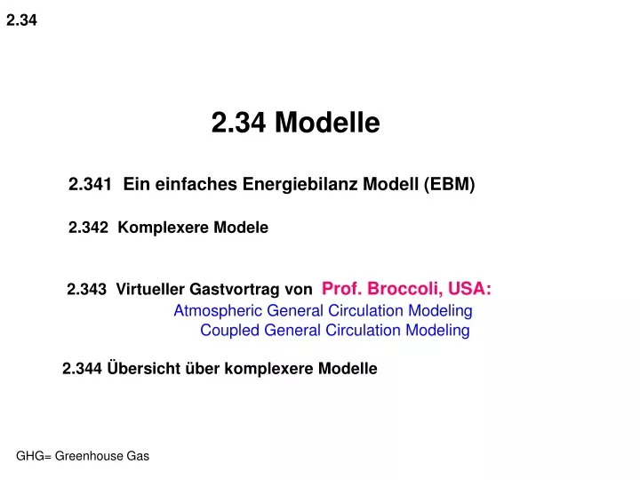
2.34. 2.34 Modelle 2.341 Ein einfaches Energiebilanz Modell (EBM) 2.342 Komplexere Modele 2.343 Virtueller Gastvortrag von Prof. Broccoli, USA: Atmospheric General Circulation Modeling Coupled General Circulation Modeling 2.344 Übersicht über komplexere Modelle.

E N D
2.34 2.34 Modelle 2.341 Ein einfaches Energiebilanz Modell (EBM) 2.342 Komplexere Modele 2.343 Virtueller Gastvortrag von Prof. Broccoli, USA:Atmospheric General Circulation Modeling Coupled General Circulation Modeling 2.344 Übersicht über komplexere Modelle GHG= Greenhouse Gas
F0 Fa Fa Tg Ground 2.341 A simple model of the greenhouse effect FS = 1370 [W/m^2]solar constant F0 = 1/4 * (1-A)* FS t*Fg thermal transmittance t Ta Atmosphere Solar transmittance s thermal emittance = (1- t ) Fa = (1-t )* Ta4 Fg = Tg4 s*F0 Fg Quelle:D.G. Andrews:“An introduction to Atmospherical Physics; fig.1.2
F0 Fa Fa Tg Ground A simple model of the greenhouse effect: Bilance at the top of the atmosphere:F0 = Fa +t*Fg (1) t*Fg thermal transmittance t Atmosphere Ta Solar transmittance s thermal emittance = (1- t ) [Kirchhoff‘s law] s*F0 Bilance at the ground:s*F0 + Fa = Fg(2) Fg Quelle:D.G. Andrews:“An introduction to Atmospherical Physics; fig.1.2
A simple model of the greenhouse effect: Bilance at the top of the atmosphere: (1)F0 = Fa+t*Fg Bilance at the ground: (2) Fg= Fa + s*F0 Faaus (1)in (2) einsetzen : Fg= [F0-t*Fg]+ s*F0 Fg= F0 * (1+ s) / ( 1+t) andererseits gilt: Fg = Tg4 Also :Tg4= F0 * (1+ s) / ( 1+t) Quelle:D.G. Andrews:“An introduction to Atmospherical Physics; fig.1.2
A simple model of the greenhouse effect: Also :Tg4 = F0 * (1+ s) / ( 1+t) Zahlenwerte:s = 0,9 ; t = 0,2 ; Albedo A=0,3 ferner: F0 = 1/4 * (1-A)* FS = 0,7* 1370/ 4 = 0,7* 340 = 240 [W/m2] = 5,67 *10- 8 [Wm-2K-4] Tg= 286 [K] The close agreement with Tg= 288 [K] is partly fortuitous,since in reality non radiative processes also contribute to the energy balance Quelle:D.G. Andrews:“An introduction to Atmospherical Physics; fig.1.2
2.342 Komplexere Modelle Komplexere Modelle
Geographic resolution characteristic of climate Models of the generations of climate models used in the IPCC Assessment Re-ports: FAR (IPCC, 1990), SAR (IPCC, 1996), TAR (IPCC, 2001a), and AR4 (2007). The figures above show how successive generations of these global models increasingly resolved northern Europe. These illustrations are representative of the most detailed horizontal resolution used for short-term climate simulations. The century-long simulations cited in IPCC Assessment Reports after the FAR were typically run with the previous generation’s resolution. Vertical resolution in both atmosphere and ocean models is not shown, but it has increased comparably with the horizontal resolution, beginning typically with a single-layer slab ocean and ten atmospheric layers in the FAR and progressing to about thirty levels in both atmosphere and ocean. Quelle: IPCC-AR4-wg1 (2007), Figure 1.4
Geographic resolution characteristic of climate Models Quelle: IPCC-AR4-wg1 (2007), Figure 1.4
aktueller Stand (2007): 30 levels in both atmosphere and ocean. Quelle: IPCC-AR4-wg1 (2007), Figure 1.4
Hierarchie der gekoppelten Modelle für Ozean und Atmosphäre nach Raumdimensionen geordnet Quelle: Prof. T. Stocker: „Einführung in die Klimamodellierung“, Vorlesungsskript WS 2002/2003; p.19; Tab.2.1 :
Erläuterungen zur Tabelle 2.1(Hierarchie der gekoppelten Modelle für Ozean und Atmosphäre ): Die Richtung der Dimensionen ist in Klammern spezifiziert: (lat = latitude, long = longitude, z = vertikal); 2.5d = mehrere 2-dimensionale Ozeanbecken, die im südlichen Ozean verbunden sind; Weitere viel verwendete Abkürzungen: EBM = energy balance model, AGCM = atmospheric general circulation model, OGCM = ocean general circulation model . QG = für quasi-geostrophisch, SST = sea surface temperature. In kursiv sind einige Modellbeispiele genannt (entweder Autoren oder Modellbezeichnung). EMICS: Das grau schattierte Gebiet enthält Klimamodelle reduzierter Komplexität (auch Earth System Models of Intermediate Complexity, EMICs genannt), mit denen lange Integrationen durchgeführt werden können (mehrere 10^3 – 10^6 Jahre, oder grosse ensembles). Quelle: Prof. T. Stocker: „Einführung in die Klimamodellierung“, Vorlesungsskript WS 2002/2003; p.19; Tab.2.1 :
Klimamodelle sind gar nicht so einfach zu verstehen und zu beurteilen (hmm…..- was tun?) Daher : 1. Hinweis auf ausführliche Vorlesungen im wwwund auf gedruckte Publikationen. 2. Virtueller Gastvortrag : Prof. Broccoli, Rutgers University, New Jersey, USA
Prof. Stocker, Bern http://www.climate.unibe.ch/ ~stocker/papers/skript0203.pdf zum Original
Inhalt der Vorlesung von Prof. Stocker 1 Einführung.................... .........................................................................................................1 1.1 Ziel der Vorlesung und weiterführende Literatur ................................................................1 1.2 Das Klimasystem..................................................................................................................3 1.3 Aufgaben und Grenzen der Klimamodellierung ..................................................................6 1.4 Historische Entwicklung ......................................................................................................9 1.5 Einige aktuelle Beispiele zur Klimamodellierung .............................................................13 1.6 Zusammenfassung.................................................................... ...........................17 2 Modellhierarchie und einfache Klimamodelle ..................................................................19 2.1 Hierarchie der physikalischen Klimamodelle ....................................................................19 2.2 Punktmodell der Strahlungsbilanz ....................................................................................27 2.3 Numerische Lösung einer gewöhnlichen Differentialgleichung 1. Ordnung ............. .......30 2.4 Klimasensitivität im Energiebilanzmodell ................................................................... ......34 3 Advektion, Diffusion und Konvektion................................................................................41 3.1 Advektion..........................................................................................................................41 3.2 Diffusion............................................................................................................................42 3.3 Konvektion........................................................................................................................43 3.4 Advektions-Diffusionsgleichung und Kontinuitätsgleichung....................... .....................44 3.5 Numerische Lösung der Advektions-Gleichung ................................................................45 3.6 Weitere Verfahren zur Lösung der Advektions-Gleichung ..................................... ..........53 3.7 Numerische Lösung der Advektions-Diffusions Gleichung ..................................... .........59 3.8 Numerische Diffusion .......................................................................................................59 4 Energietransport im Klimasystem und seine Parametrisierung .....................................61 4.1 Grundlagen........................................................................................................................61 4.2 Wärmetransport in der Atmosphäre ..................................................................................62 4.3 Breitenabhängiges Energiebilanzmodell............................................................................65 4.4 Wärmetransport im Ozean ................................................................................................66 .......................................................
5 Anfangswert- und Randwertprobleme...............................................................................71 5.1 Allgemeine Grundlagen .....................................................................................................71 5.2 Direkte numerische Lösung der Poissongleichung ............................................................72 5.3 Iterative Verfahren .............................................................................................................74 5.4 Successive Overrelaxation (SOR)......................................................................................75 6 Gross-skalige Zirkulation im Ozean...................................................................................77 6.1 Die Bewegungsgleichungen......................................................................................... .....77 6.2 Flachwassergleichungen als Spezialfall ............................................................................80 6.3 Verschiedene Typen von Gittern in Klimamodellen........................................................ ..81 6.4 Spektralmodelle.................................................................................................................85 6.5 Windgetriebene Strömung im Ozean (Stommel Modell) .............................................. ...87 6.6 Potentielle Vorticity: eine wichtige Erhaltungsgrösse .................................................... ..93 7 Gross-skalige Zirkulation in der Atmosphäre ..................................................................97 7.1 Zonale und meridionale Zirkulation .............................................................................. ....97 7.2 Das Lorenz-Saltzman Modell ..........................................................................................102 8 Atmosphäre-Ozean Wechselwirkung...............................................................................109 8.1 Kopplung von physikalischen Modellkomponenten................................................... .....109 8.2 Thermische Randbediungungen.................................................................................. .....110 8.3 Hydrologische Randbedingungen............................................................................... .....114 8.4 Impulsflüsse ............................................................................................................. ........116 8.5 Gemischte Randbedingungen ................................................................................... .......116 8.6 Gekoppelte Modelle................................................................................................... .. ...118 9 Multiple Gleichgewichte im Klimasystem .......................................................................122 9.1 Abrupte Klimawechsel aufgezeichnet in polaren Eisbohrkernen ............................... .....122 9.2 Multiple Gleichgewichte in einem einfachen Atmosphärenmodell............................. ....124 9.3 Multiple Gleichgewichte in einem einfachen Ozeanmodell ....................................... .....125 9.4 Multiple Gleichgewichte in gekoppelten Modellen.................................................... .....127 9.5 Schlussbemerkungen und Ausblick .................................................................................130 10 Übungsaufgaben zur Klimamodellierung........................................................................131
Prof. Claussen, Potsdam http://www.pik-potsdam.de/ ~claussen/lectures/ physikalische_klimatologie/ physklim1.pdf zum Original
IMPRS, 4 June 2003 Earth System Models of Intermediate Complexity 1. Martin Claussen Potsdam-Institut für Klimafolgenforschung / Universität Potsdam • Remarks on the Earth system • The spectrum of Earth system models • Examples from CLIMBER-2 and EMIC workshops • Perspective for Integrative Modelling Quelle: Claussen: „Earth System Models of Intermediate Complexity“,IMPRS, 4.6.2003; www.pik-potsdam.de/~claussen/lectures/
Climate modelling with quasi-realistic models - experiences in describing climate during the Holocene and the Eemian, and in designing scenarios of plausible future climate change. The construction and utility of quasi-realistic climate models is reviewed. Examples of reconstructing past climates are presented, in particular for the last millennium and for the last interglacial, the Eemian (120 ka bp). In addition, the approach of constructing plausible future climates, conditional upon the extent the atmosphere is used as a dump for anthropogenic substances, is demonstrated with examples. Hans von StorchInstitute for Coastal Research, GKSS Research Center, Geesthacht, Germany Prof. von Storch, GKSS Quelle: Hans von Storch: „Climate modelling with quasi-realistic models..”, Vortrag Madrid 7.5.2004; http://w3g.gkss.de/G/Mitarbeiter/storch/ 7.5.2004 Centro de Astrobiología, Madrid http://w3g.gkss.de/G/Mitarbeiter/storch/
2. Virtueller Gastvortrag zunächst: Vorbereitung und Einstimmung
Die Atmosphäre über Europa im diskreten Modell U. Cubasch BQuelle:DLR_Schumann200_Klimawandel.ppt
Europa im diskretisierten Modell U. Cubasch BQuelle:DLR_Schumann2000_Klimawandel.ppt
McGuffie and Hendersson-Sellers, 1997 BezugsQuelle: Claussen: „Earth System Models of Intermediate Complexity“,IMPRS, 4.6.2003; www.pik-potsdam.de/~claussen/lectures/
Für die zeit- und ortsabhängigen Zustandsvariablen: T = Temperatur = Dichte p = Druck {u,v,w} = Strömungsgeschwindigkeit (3 Komponenten) gelten in jeder Zelle die Grundgleichungen der Strömungs- undThermodynamik. (Erhaltung von Impuls [NavierStokes], Masse [Kontinuitätsgleichung], und Energie, und Zustandsgleichung .) Im Ozean wird an Stelle der Dichte meist der Salzgehalt S benutzt, da: = (S,T,p) . In der Atmosphäre kommen noch wg. der Energiebilanz der Wasserdampfgehalt q und flüssiges Wolkenwasser hinzu. Quelle: / Storch-Güss-Heimann 99, p.99ff./
Es wird ein auf der rotierenden Erde (Corioliskraft! ) ortsfestes (Advektionsterm! ) Koordinatensystem verwendet. Daher treten in den Navier Stokes Gln.(Impulserhaltung) auf: der Coriolis Parameter f:f = 2 ** sin mit: = Winkelgeschwindigkeit der Erddrehung , = geographische Breite und länge der Erdradius : a Quelle: / Storch-Güss-Heimann 99, p.99ff./
Erinnerung an die Hydrodynamik: Eulerian and Lagrangian description BQuelle: Prof. Dick Yue,MIT_ocw 13.021 „Marine Hydrodynamics“, lecture notes „2 Basic Equations“ http:/ocw.mit.edu/OcwWeb/Ocean-Engineering/13-021MarineHydrodynamicsFall2001/CourseHome/index.htm
Behauptung : Es gilt: Erinnerung an die Hydrodynamik:D /Dt BQuelle: Prof. Dick Yue,MIT_ocw 13.021
atmosphere Quelle: v.Storch: „Climate modelling with quasi-realistic models..”, Vortrag Madrid 7.5.2004; http://w3g.gkss.de/G/Mitarbeiter/storch/
ocean Quelle: v.Storch: „Climate modelling with quasi-realistic models..”, Vortrag Madrid 7.5.2004; http://w3g.gkss.de/G/Mitarbeiter/storch/
Parameterizations The terms Fu, Fv, Gq,Gs, GTandQ describe the effect of “unresolved” processes on state variables u, v, q, ρ and T, i.e.,Fu = Fu,Δx(u, v, q, ρ,T) These functions are called „parameterizations“; they are not uniquely determined (i.e., different formulations may serve the same purpose), and the limiting process is not defined, i.e., Fu,Δx(u, v, q, ρ,T) does not exist. There is nothing like “the differential equations” of climate. Quelle: v.Storch: „Climate modelling with quasi-realistic models..”, Vortrag Madrid 7.5.2004; http://w3g.gkss.de/G/Mitarbeiter/storch/
Institut für Küstenforschung I f K Dynamical processes in the atmosphere Quelle: v.Storch: „Climate modelling with quasi-realistic models..”, Vortrag Madrid 7.5.2004; http://w3g.gkss.de/G/Mitarbeiter/storch/
Institut für Küstenforschung I f K Dynamical processes in a global atmospheric model Quelle: v.Storch: „Climate modelling with quasi-realistic models..”, Vortrag Madrid 7.5.2004; http://w3g.gkss.de/G/Mitarbeiter/storch/
Institut für Küstenforschung I f K Dynamical processes in the ocean Quelle: v.Storch: „Climate modelling with quasi-realistic models..”, Vortrag Madrid 7.5.2004; http://w3g.gkss.de/G/Mitarbeiter/storch/
Institut für Küstenforschung I f K Dynamical processes in a global ocean model Quelle: v.Storch: „Climate modelling with quasi-realistic models..”, Vortrag Madrid 7.5.2004; http://w3g.gkss.de/G/Mitarbeiter/storch/
Quasi-realistic Models • Models of aximum complexity, which feature as many processes as is possible given the computational resource. • Meant as a tool to simulate in space-time detail the trajectory of climate. • Quasi-realistic models do not “explain” but allow for “numerical experiments”. Quelle: Hans von Storch: „Climate modelling with quasi-realistic models..”, Vortrag Madrid 7.5.2004; http://w3g.gkss.de/G/Mitarbeiter/storch/
Quasi-realistic models Quelle: Hans von Storch: „Climate modelling with quasi-realistic models..”, Vortrag Madrid 7.5.2004; http://w3g.gkss.de/G/Mitarbeiter/storch/
2.343 Virtueller Gastvortrag von Prof. Broccoli, USA: 1. Atmospheric General Circulation Modeling 2. Coupled General Circulation Modeling Prof. Anthony J. Broccoli Dept. of Environmental Sciences Rutgers University, New Jersey, USA Homepage: http://www.envsci.rutgers.edu/~broccoli/index.html
Atmospheric General Circulation Modeling Anthony J. BroccoliDept. of Environmental Sciences Zum Original:http://climate.envsci.rutgers.edu/climod/BroccoliAtmos_gcm_env544.ppt
Coupled General Circulation Modeling Anthony J. BroccoliDept. of Environmental Sciences Zum Original: http://climate.envsci.rutgers.edu/climod/BroccoliCoupled_gcm_env544.ppt
Ist dies Bild schöner als die Urfassung,das folgende Bild? 2.344 Übersicht : Komplexere Modelle
Box 3: Climate Models: How are they built and how are they applied? Comprehensive climate models are based on physical laws represented by mathematical equations that are solved using a three-dimensional grid over the globe. For climate simulation, the major components of the climate system must be represented in submodels (atmosphere, ocean, land surface, cryosphere and biosphere), along with the processes that go on within and between them. Most results in this report are derived from the results of models, which include some represen-tation of all these components. Global climate models in which the atmosphere and ocean components have been coupled together are also known as Atmosphere-Ocean General Circulation Models (AOGCMs). In the atmospheric module, for example, equations are solved that describe the large-scale evolution of momentum, heat and moisture. Similar equations are solved for the ocean. Currently, the resolution of the atmospheric part of a typical model is about 250 km in the horizontal and about 1 km in the vertical above the boundary layer. The resolution of a typical ocean model is about200 to 400 m in the vertical, with a horizontal resolution of about 125 to 250 km. Equations are typically solved for every half hour of a model integration. Many physical processes, such as those related to clouds or ocean convection, take place on much smaller spatial scales than the model grid and therefore cannot be modelled and resolved explicitly. Their average effects are approximately included in a simple way by taking advantage of physically based relationships with the larger-scale variables. This technique is known as parametrization. IPCC2001_TAR1_TS-Box3
2.35 Projektionen und Szenarios für das 21. Jahrhundert