Download
1 / 34
340 likes | 408 Views
Bayesian Estimators of Time to Most Recent Common Ancestry. Bruce Walsh. jbwalsh@u.arizona.edu. Ecology and Evolutionary Biology. Adjunct Appointments Molecular and Cellular Biology Plant Sciences Epidemiology & Biostatistics Animal Sciences.

E N D
Bayesian Estimators ofTime to Most Recent Common Ancestry Bruce Walsh jbwalsh@u.arizona.edu Ecology and Evolutionary Biology Adjunct Appointments Molecular and Cellular Biology Plant Sciences Epidemiology & Biostatistics Animal Sciences
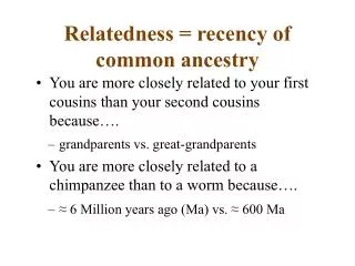
Problem: Given some genetic marker information for a pair of individuals, what can we say about how recently they are related? Application in Genealogy -- how closely are (say) Bill Walsh (former football coach) and I related? Basic concept: The more closely related, the more genetic markers in common we should share For forensic applications: 11 highly polymorphic Automosomal marker loci sufficient for individualization Measure relatedness by TMRCA, the time to the most Recent common ancestor (MRCA)
Often we are very interested in TMRCAs that are modest (5-10 generations) or large (100’s to 10,000’s of generations) Unlinked autosomal markers simply don’t work over these time scales. Reason: With autosomes, unlinked markers assort each generation leaving only a small amount of IBD information on each marker, which we must then multiply together. IBD information decays on the order of 1/2 each generation. To extract the signal for 5-10 generations would require a very large number of automosomal markers (order of 100’s)
Y Chromosomes How then can we accurately estimate TMRCA for modest to large number of generations? Answer: Use a set of completely linked markers, such as those on the nonrecombiming arm of the Y chromosome. With completely linked marker loci, information on IBD does not assort away via recombination. IBD information decay is on the order of the mutation rate, roughly 1/250 - 1/500 per generation.
Infinite Alleles Model The first step in estimating TMRCA requires us to assume a particular mutational model Our (initial) assumption will be the infinite alleles model (IAM) The key assumption of this model (originally due to Kimura and Crow, 1964) is that each new mutation gives rise to a new allele.
A B (1-u)t (1-u) t Pr(No mutation from MRCA->A) = (1-u)t Pr(No mutation from MRCA->B) = (1-u)t MRCA MRCA Key: Under the infinite alleles, two alleles that are identical in state that are also ibd have not experienced any mutations since their MRCA. Let q(t) = Probability two alleles with a MRCA t generations ago are identical in state If u = per generation mutation rate, then q(t) = (1-u)2t
Building the Likelihood Function for n Loci The probability that k of n marker loci are IBS is just a Binomial distribution with success parameter q(t) Likelihood function for t given k of n matches - - - - - ( - ) - - For any single marker locus, the probability of IBS given a TMRCA of t generations is q(t) = (1-u)2t ≈ e-2ut = e-t, t = 2ut
MLE for t is solution of ∂ L/∂t = 0 ( ) ( ) ^ - - ^ - ( - ) - - p = fraction of matches ML Analysis of TMRCA It would seem that we now have all the pieces in hand for a likelihood analysis of TMRCA given the marker data (k of n matches) Likelihood function (t = 2ut)
( ) - Likewise, the precision of this estimator follows for the (negative) inverse of the 2nd derivative of the log-likelihood function evaluated at the MLE, ( ) - - ^ - Var( t ) = ^ In particular, the MLE for t becomes
Trouble in Paradise The ML machinery has seem to have done its job, giving us an estimate, its approximate sampling error, approximate confidence intervals, and a scheme for hypothesis testing. Hence, all seems well. Problem: Look at k=n (= complete match at all markers). MLE (TMRCA) = 0 (independent of n) Var(MLE) = 0 (ouch!) The one-LOD support interval is from t=0 to t = (1/2n) [ -Ln(10)/Ln(1-u) ] = (0, 575/n)
MLE(t) = 0 for all values on n 1 LOD ≈ t = 29 1 LOD ≈ t = 58 1 LOD ≈ t = 115 0.1 of max value (1) of likelihood function With n=k, likelihood function reduces to L(t) = (1-u)2tn ≈ e-2tun n=5 n=10 L(t) n=20 t (Plots for u = 0.002)
The problem(s) with ML The expressions developed for the sampling variance, approximate confidence intervals, and hypothesis testing are all large-sample approximations Problem 1: Here our sample size is the number of markers scored in the two individuals. Not likely to be large (typically 10-30). Problem 2: These expressions are obtained by taking appropriate limits of the likelihood function. If the ML is exactly at the boundary of the admissible space on the likelihood surface, this limit may not formally exist, and hence the above approximations are incorrect.
posterior distribution of q given x Likelihood function for q Given the data x priordistribution for q The appropriate constant so that the posterior integrates to one. The Solution? Go Bayesian Instead of simply estimating a point estimate (e.g., the MLE), the goal is the estimate the entire distributionfor the unknown parameter q given the data x p(q | x) = C * l(x | q) p(q) Why Bayesian? • Exact for any sample size • Marginal posteriors • Efficient use of any prior information
The Prior on TMRCA The first step in any Bayesian analysis is choice of an appropriate prior distribution p(t) -- our thoughts on the distribution of TMRCA in the absence of any of the marker data Standard approach: Use a flat or uninformative prior, with p(t) = a constant over the admissible range of the parameter. Can cause problems if the likelihood function is unbounded (integrates to infinity) In our case, population-genetic theory provides the prior: under very general settings, the time to MRCA for a pair of individuals follows a geometric distribution
Prior hyperparameter = 1/Ne - - - - Previous likelihood function (ignoring constants that cancel when we compute the normalizing factor C) Prior In particular, for a haploid gene, TMRCA follows a geometric distribution with mean 1/Ne. Hence, our prior is just p(t) = l(1-l)t≈l e-lt, where l = 1/Ne Hence, we can use an exponential prior with hyperparameter (the parameter fully characterizing the distribution) l = 1/Ne. The posterior thus becomes
- - - - - - - - The Normalizing constant where I ensures that the posterior distribution integrates to one, and hence is formally a probability distribution
- - - - What is the effect of the hyperparameter? If 2uk >> l, then essentially no dependence on the actual value of l chosen. Hence, if 2Neuk >> 1, essentially no dependence on (hyperparameter) assumptions of the prior. For a typical microsatellite rate of u = 0.002, this is just Nek >> 250, which is a very weak assumption. For example, with k =10 matches, Ne >> 25. Even with only 1 match (k=1), just require Ne >> 250.
- - - - - ( - - - - = - - - - - - - - Closed-form Solutions for the Posterior Distribution Complete analytic solutions to the prior can be obtained by using a series expansion (of the (1-ex)n term) to give Each term is just a * ebt, which is easily integrated
- - - - - - - - - - - - - - - - - - With the assumption of a flat prior, l = 0, this reduces to
( - - - - - - - - - Hence, the complete analytic solution of the posterior is Suppose k = n (no mismatches) In this case, the prior is simply an exponential distribution with mean 2un + l,
< - - - - Analysis of n = k case Mean TMRCA and its variance: Cumulative probability: In particular, the time Ta satisfying P(t < Ta) = a is
For a flat prior (l = 0), the 95% (one-side) confidence interval is thus given by -ln(0.5)/(2nu) ≈ 1.50/(nu) Hence, under a Bayesian analysis for u = 0.002, the 95% upper confidence interval is given by ≈ 749/n Recall that the one-LOD support interval (approximate 95% CI) under an ML analysis is ≈ 575/n The ML solution’s asymptotic approximation significantly underestimates the true interval relative to the exact analysis under a full Bayesian model
Posteriors for n = 10 Posteriors for n = 20 Posteriors for n = 50 n = 100 93 n = 100 0.30 92 0.060 94 91 100 90 0.25 0.050 99 0.20 0.040 p( t | k ) p( t | k ) 98 89 0.15 97 0.030 96 95 0.10 0.020 0.05 0.010 0.00 0.000 1 2 3 4 5 6 7 8 9 10 11 12 13 14 15 16 17 18 19 20 0 5 10 15 20 25 30 35 40 45 50 55 60 65 Time t to MRCA Time t to MRCA Sample Posteriors for u = 0.002
Key points • By using markers on a non recombining chromosomal section, we can estimate TMRCA over much, much longer time scales than with unlinked autosomal markers • By using the appropriate number of markers we can get accurate estimates for TMRCA for even just a few generations. 20-50 markers will do. • Hence, we have a fairly large window of resolution for TMRCA when using a modest number of completely linked markers.
Mutation 1 Mutation 2 Under IAM, score as a match, and hence no mutations In reality, there are two mutations Stepwise Mutation Model (SMM) Microsatellite allelic variants are scored by their number of repeat units. Hence, two “matching” alleles can actually hide multiple mutations (and hence more time to the MRCA) The Infinite alleles model (IAM) is not especially realistic with microsatellite data, unless the fraction of matches is very high.
- - > - ( ) Formally, the SMM model assumes the following transition probabilities Note that two alleles can match only if they have experienced an even number of mutations in total between them. In such cases, the match probabilities become
- ( - The zero-order modifed Type I Bessel Function ( ) - Hence,
Under the SMM model, the prior hyperparameter can now become important. This is the case when the number n of markers is small and/or k/n is not very close to one Why? Under the prior, TMRCA is forced by a geometric with 1/Ne. Under the IAM model for most values this is still much more time than the likelihood function predicts from the marker data Under the SMM model, the likelihood alone predicts a much longer value so that the forcing effect of the initial geometric can come into play
n =5, k = 3, u = 0.02 IAM, both flat prior and Ne = 5000 SSMO, Ne = 5000 SSMO, flat prior Pr(TMRCA < t) Prior with Ne =5000 Time, t
> - The jth-order modifed Type I Bessel Function … … An Exact Treatment: SMME With a little work we can show that the probability two sites differ by j steps is just The resulting likelihood thus becomes Where nj is the number of sites that differ by k (observed) steps
… - - … - Number of exact matches Number of k steps differences With this likelihood, the resulting prior becomes This rearranges to give the general posterior under the Exact SMM model (SMME) as
Example Consider comparing haplotypes 1 and 3 from Thomas et al.’s (2000) study on the Lemba and Cohen Y chromosome modal haplotypes. Here six markers used, four exactly match, one differs by one repeat, the other by two repeats Hence, n = 6, k = 4 for IAM and SMM0 models n0 = 4, n1 = 1, n2 = 1, n = 6 under SMME model Assume Hammer’s value of Ne=5000 for the prior
IAM SMM0 P(t | markers) SMME Time to MRCA, t TMRCA for Lemba and Cohen Y
IAM SMM0 Pr(TMRCA < t) SMME Time to MRCA, t