Download
1 / 48
490 likes | 708 Views
Chapter 11 Cost benefit analysis. 11.1 Intertemporal welfare economics 11.2 Project appraisal 11.3 Cost-benefit analysis and the environment Learning objectives learn about the conditions necessary for intertemporal efficiency

E N D
Chapter 11 Cost benefit analysis 11.1 Intertemporal welfare economics 11.2 Project appraisal 11.3 Cost-benefit analysis and the environment Learning objectives learn about the conditions necessary for intertemporal efficiency §revisit the analysis of optimal growth introduced in Chapter 3 §find out how to do project appraisal §learn about cost–benefit analysis and its application to the environment §be introduced to some alternatives to cost–benefit analysis
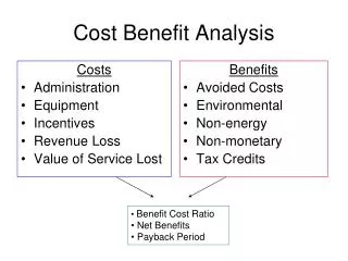
Cost-benefit analysis Cost-benefit analysis, CBA, is the social appraisal of marginal investment projects, and policies, which have consequences over time It uses criteria derived from welfare economics, rather than commercial criteria. CBA seeks to correct project appraisal for market failure Environmental impacts of projects/policies are frequently externalities, both negative and positive CBA seeks to attach monetary values to external effects so that they can be taken account of along with the effects on ordinary inputs and outputs to the project/policy CBA is the same as BCA – Benefit-cost analysis.
Intertemporal efficiency Given that CBA is concerned with consequences over time, and based in welfare economics, a key idea is that of intertemporal efficiency. (11.1) An allocation is efficient if it is impossible to make one individual better off without thereby making the other worse off. Intertemporal efficiency requires the satisfaction of 3 conditions Equality of individuals’ consumption discount rates Equality of rates of return to investment across firms Equality of the common consumption discount rate with the common rate of return
Discount rate equality = otherwise one could be made better off without making the other worse off MRUS MRUS ≡ defines A’s consumption discount rate Then the first intertemporal efficiency condition is stated as rA=rB = r (11.2) Note: consumption discount rates are not constants.
Shifting consumption over time Foregoing Cb0Ca0 makes Ca1Cb1 available next period. The rate of return to, on,investment is defined as where ΔC1 is the second period increase in consumption, Ca1Cb1, resulting from the first period increase in investment ΔI0, Cb0Ca0. For ΔI0 = ΔC0, this is which is the negative of the slope of the transformation frontier minus 1, which can be written where s is the slope of the frontier.
Rate of return equality If each firm were investing as indicated by C01b and C02b, then period 1 consumption could be increased, without loss of period 0 consumption, by having firm 1, where the rate of return is higher, increase investment by the amount firm 2, where the rate of return is lower, reduced its investment. Only where rates of return are equal is this kind of period 1 gain impossible. For N firms, the second intertemporal efficiency condition is (11.3)
Equality of discount rate and rate of return If the first two conditions are satisfied, we can consider representative individual and firm. Point a corresponds to intertemporal efficiency, b and c do not as from either could reallocate consumption as between periods so as to move on to a higher consumption indifference curve. At a the slopes of the consumption indifference curve and the consumption ttansformation frontier are equal. The third condition is (11.4)
Intertemporal optimality As in the single period situation, the intertemporal efficiency conditions do not fix a unique intertemporal allocation. That requires a social welfare function with utilities as arguments Will consider this under ‘Optimal growth models’
Markets and intertemporal efficiency – futures markets Futures Markets X at t is treated as a different commodity from X and t+1 For N commodities and M periods there are MN dated commodities. Contracts are written at the start of the first period for trades an all commodities at all future dates. Then, it is effectively the static case. Given that all ideal circumstances apply in all MN markets, the conditions for intertemporal efficiency will be satisfied. Futures markets are, in fact, rare – standardised raw materials, financial instruments.
Markets and intertemporal efficiency – loanable funds market Loanable Funds Market x is the bond coupon paid on the first day of period 1 Pb is the price the bond trades for on the first day of period 0 i is the interest rate A seller is a borrower A buyer is a lender
Individuals - utility maximisation UU is a consumption indifference curve, slope –(1+r) Line C1max C0max is the budget constraint, slope –(1+i) Optimum is at C*0 in period 0 and C*1 in period 1, where r = i which will hold for all individuals, satisfying the first intertemporal efficency condition
Firms – present value maximisation Owners of firms can shift consumption by investing in firm dealing in the bond market AB shows C0 C1 combinations on account of varying investment, slope –(1+ δ), δ is the rate of return to investment RS with slope -(1+i) shows how consumption can be shifted via bond market dealing. The optimum level of investment is at a, where the present value of the firm is maximised, and where i = δ In the second stage the owner maximises utility, by bond market dealing, at b where i = r All owners so act, and the three conditions for intertemporal efficiency are satisfied.
Optimal growth modelling; discrete time A representative individual model for two periods Maximise (11.5a) subject to Q0(K0) – (K1 – K0) = C0 (11.5b) Q1(K1) – (K2 – K1) = C1 (11.5c) Here the efficiency problem is trivial – consumption in one period can only be increased by reducing it in the other period. A necessary condition is (11.6) So with diminishing marginal utility, C1 greater than C0 implies that ρ (the utility discount rate) is less then δ (the rate of return on investment). For ρ = δ, consumption is constant.
Optimal growth modelling: continuous time Maximise (11.7a) Subject to = Q(Kt) - Ct (11.7b) has necessary condition (11.8) where ρ is a parameter, the utility discount rate, and δ is a variable, the rate of return to capital accumulation. For δ > ρ, given diminishing marginal utility, C is growing. Consumption growth ceases when δ = ρ.
A model with resource input to production Maxximise (11.9a) Subject to (11.9b) (11.9c) In this model intertemporal efficiency is not trivial. There are two forms of investment, in capital and in the resource stock. Efficiency requires that the rates of return on the two are equal. See chapter 14 especially
Utility and consumption discount rates 1 Figure 11.8 Indifference curves in utility and consumption space intertemporal welfare function for panel a slope of WCWC in panel b (11.10)
Utility and consumption discount rates 2 In continuous time (11.11) where r is the consumption discount rate ρ is the utility discount rate η is is the elasticity of marginal utility for the instantaneous utility function g is the growth rate For g>0 r> ρ and r would be positive for ρ = 0 For g = 0 r = ρ
Private project appraisal – the Net Present Value test 1 The present value of expenditures E is (11.14) The present value of receipts R is (11.15) The present value of the project is (11.16) Which for N = R - E is (11.17) The project should go ahead iff NPV≥0
Private project appraisal – the Net Present Value test 2 Year Expenditure Receipts Net cash flow 0 100 0 –100 1 10 50 40 2 10 50 40 3 10 45.005 35.005 4 0 0 0 Table 11.2 Example net cash flow 1 at i = 0.05, NPV = £4.6151 at i = 0.075, NPV = £0 at i = 0.10, NPV = -£4.27874 The NPV of a project is the amount by which it increases the firm’s net worth. It is the present value of the surplus, after financing the project, at the end of the project lifetime.
Private project appraisal - risk Year Year Expected net cash flow Net cash flow 1 Probability 0.6 Present value of expected cash flow Net cash flow 2 Probability 0.4 0 0 –(0.6 x 100) + {–(0.4 x 100)} = –100 –100 –100 –100 1 1 (0.6 x 40) + (0.4 x 35) = 38 40 38/1.075 = 35.35 35 2 2 (0.6 x 40) + (0.4 x 35) = 38 40 38/1.0752 = 32.88 35 3 3 (0.6 x 35.005) + (0.4 x 25) = 31.003 35.005 31.003/1.0753 = 24.96 25 4 4 (0.6 x 0) + (0.4 x 0) = 0 0 0 Expected NPV –6.81 Table 11.4 One project, two possible cash flows Table 11.5 Calculation of expected NPV Where the firm is prepared to assign probabilities, the criterion for going ahead with the project is the expected NPV – the probability weighted sum of the mutually exclusive cash flow outcomes. This assumes that the decision maker is risk-neutral Chapter 13 on decision making in the face of imperfect knowledge of the future.
Social project appraisal CBA is the social appraisal of projects CBA uses the NPV test CBA can be approached in two ways As an extension of private appraisal where externalities are taken into account In terms of social welfare enhancement The first stages of CBA are proper project/policy identification forecasting all of the consequences of the project/policy for all of the affected individuals in each year of the project/policy lifetime Then expressing consequences in terms of monetary gains/losses for aggregation to an NPV number
Social appraisal: an illustrative project Time period Individual 0 1 2 3 Overall A NBA,0 NBA,1 NBA,2 NBA,3 NBA B NBB,0 NBB,1 NBB,2 NBB,3 NBBB C NBC,0 NBC,1 NBC,2 NBC,3 NBC Society NB0 NB1 NB2 NB3 Table 11.6 Net benefit (NB) impacts consequent upon an illustrative project Generally, go ahead if (11.19)
CBA as a potential pareto improvement test A positive NPV indicates that, with due allowance for the dating of costs and benefits, the project delivers a surplus of benefit over cost. The consumption gains involved are greater than the consumption losses, taking account of the timing of gains and losses. The existence of a surplus means that those who gain from the project could compensate those who lose and still be better off. Finance by taxation – two periods The initial investment is ΔI0, equal to -ΔC0, and the consumption increment on account of going ahead with the project is ΔC1. First period consumers lose an amount ΔC0, equal to ΔI0, and second period consumers gain ΔC1, and the question is whether the gain exceeds the loss. From the viewpoint of the first period, the second period gain is worth ΔC1/(1+r), so the question is whether ΔC1/(1+r) > ΔI0 (11.20) is true, which is the NPV test discounting at r. Finance by borrowing – two periods The government funds the project by borrowing and the project displaces the marginal private sector project with rate of return δ. In this case the cost of the public sector project is ΔI0 in the first period plus δΔI0 in the second, this being the extra consumption that the private sector project would have generated in the second period. In this case, from the viewpoint of the first period, the gain exceeds the loss if: (11.21) This is the NPV test with the consumption gain discounted at the consumption rate of interest, and compared with the cost of the project scaled up to take account of the consumption that is lost on account of the displaced private sector project.
CBA as welfare increase test 1 Time period Individual 0 1 2 3 Overall A ΔUA,0 ΔUA,1 ΔUA,2 ΔUA,3 ΔUA B ΔUB,0 ΔUB,1 ΔUB,2 ΔUB,3 ΔUB C ΔUC,0 ΔUC,1 ΔUC,2 ΔUC,3 ΔUC Society ΔU0 ΔU1 ΔU2 ΔU3 Table 11.7 Changes in utility (∆U) consequent on an illustrative project W = W(UA,0,..., UC,3) positive – the project should go ahead Or with an intratemporal social welfare function mapping individual utilities into a social aggregate Ut W = W(U0, U1, U2, U3) positive – the project should go ahead where a widely entertained particular form is is exponential discounting
CBA as welfare increase test 2 Time period Individual 0 1 2 3 Overall A NBA,0 NBA,1 NBA,2 NBA,3 NBA B NBB,0 NBB,1 NBB,2 NBB,3 NBBB C NBC,0 NBC,1 NBC,2 NBC,3 NBC Society NB0 NB1 NB2 NB3 Utility variations consequent on going ahead with the project cannot be estimated. But, using the methods of chapter 12, monetary equivalent gains and losses can be estimated. implies (11.22) where or r = ρ + ηg (11.23) or
CBA as welfare increase test 3 The NPV test is interpreted as a test that identifies projects that yield welfare improvements - positive and negative consumption changes, net benefits that is, are added over time after discounting, so that (11.24) and for ΔW > 0 the project is welfare enhancing and should go ahead Finance by taxation two periods (11.25) where the rhs is NPV, positive for ΔC1/(1+r) > ΔI0 Finance by borrowing, two periods If the project crowds out the marginal private sector project (11.26) where the rhs is NPV, positive if
Choice of discount rate 1 Time Horizon Years Discount rate % 25 50 100 200 0.5 88.28 77.93 60.73 36.88 2 60.95 37.15 13.80 1.91 3.5 42.32 17.91 3.21 1.03 7 18.43 3.40 0.12 0.0001 There is disagreement about the discount rate that should be used in CBA This matters because the result of the NPV test can be very sensitive to the number used for the discount rate. This is especially true where the project lifetime is long, as it often is with projects with environmental consequences – the lifetime is when the longest lasting consequence ceases, not when the project stops yielding the benefits which were its purpose – nuclear electricity generation and waste products. Table 11.8 Present values at various discount rates For £100 at futurity shown
Choice of discount rate 2 With no market failure r = i = δ Given market failure which to use? Generally agreed that whichever way looking at CBA – potential pareto improvement or welfare enhancing – should use r, the consumption discount rate. Shadow pricing While it is agreed that r should be used to discount, δ appears in the NPV criterion as (11.21) and (11.26) which apply with finance by borrowing when there is crowding out – δ is there to adjust the initial cost, shadow price it, for the displacement of the marginal private sector project. At one time it was thought that, on account of crowding out, proper shadow pricing of all inputs and outputs was important in CBA. And difficult. Now the dominant view is that given international capital mobility, crowding out is not a problem – that the supply of capita for private sector projects could be treated as perfectly elastic. Shadow pricing is not now seen as necessary in CBA
Choice of discount rate 3 – descriptive versus prescriptive Regarding CBA as about potential pareto improvement aligns with the descriptive approach to determining a number for r – it should be the post tax return on risk free lending reflecting the rate at which people are willing to exchange current for future consumption. Those who regard CBA as a test for welfare enhancement tend to adopt the prescriptive approach to a number for r, according to r = ρ + ηg (11.23) where ρ is the utility discount rate η is the elasticity of the marginal utility of consumption g is the growth rate Some economists want to get values for ρ and η from observed behaviour, some from ethical considerations. Much of the controversy among economists over the Stern Review of the climate change problem focussed on the numbers used in (11.23) – Stern took an ethical prescriptive position
Box 11.2 Discount rate choices in practice Years ahead 31-75 76-125 126-200 201-300 301+ Discount rate 3.0% 2.5% 2.0% 1.5% 1.0% US Office of Management and Budget 7% as an estimate of pre-tax return on capital US Environmental Protection Agency For intragenerational – descriptive, r as 2-3% For intergenerational - r = ρ + ηg with ρ = 0 on ethical grounds, gives r 0.5% to 3% HM Treasury UK ‘Green Book’ instructions based on r = ρ + ηg – ‘evidence’ suggests ρ = 1.5%, η = 1 and g = 2% giving r = 3.5%. For lifetimes greater than 30 years because of ‘uncertainty about the future’ The Stern Review Implicit r of 2.1% from r = ρ + ηg with ρ = 0.1%, η = 1, and g = 2%.
Environmental cost-benefit analysis Look at wilderness area development. With Bd for development benefits and Cd for development costs, and ignoring environmental impact Denote this as NPV’. Then the proper NPV taking account of environmental impacts is NPV = Bd – Cd – EC = NPV’ – EC (11.27) where EC is the present value of the stream of the net value of the project’s environmental impacts over the lifetime of the project. EC stands for Environmental Cost From (11.27) the project should go ahead if NPV’ = Bd – Cd > EC (11.28)
Inverse ECBA A wilderness development project should not go ahead if EC ≥ NPV’ = Bd – Cd so that EC* = NPV’ = Bd – Cd (11.29) defines a threshold value for EC. For EC ≥ EC* the project should not go ahead. The exercises ( Chapter 12 ) that seek to ascertain EC are typically expensive, and sometimes controversial. Consideration of EC* can put their results in perspective. As can consideration of EC*/N, where N is the size of the relevant affected population, which is not necessarily restricted to visitors, and may include people from a wider area than the host country, as with an internationally recognised wilderness/ conservation area inscribed as ‘world heritage’.
Box 11.3 Mining at Coronation Hill? In 1990 there emerged a proposal to develop a mine at Coronation Hill in the Kakadu national park, which is listed as a World Heritage Area. The Australian federal government referred the matter to the Resource Assessment Commission, which undertook a very thorough exercise in environmental valuation using the Contingent valuation Method, implemented via a survey of a sample of the whole Australian population. This exercise produced a range of estimates for the median willingness to pay, WTP, to preserve Coronation Hill from the proposed development, the smallest of which was $53 per year. If it is assumed, conservatively, that the $53 figure is WTP per household, and this annual environmental damage cost is converted to a present value capital sum in the same way as the commercial NPV for the mine was calculated, the EC to be compared with the mine NPV' is, in round numbers, $1500 million. This 'back of the envelope' calculation assumes 4 million Australian households, and a discount rate of 7.5%. It was pointed out that given the small size of the actual area directly affected, the implied per hectare value of Coronation Hill greatly exceeded real estate prices in Manhattan, whereas it was 'clapped out buffalo country' of little recreational or biological value. In fact, leaving aside environmental considerations and proceeding on a purely commercial basis gave the NPV' for the mine as $80 million, so that the threshold per Australian household WTP required to reject the mining project was, in round numbers, $3 per year, less than one-tenth of the low end of the range of estimated household WTP on the part of Australians. Given that Kakadu is internationally famous for its geological formations, biodiversity and indigenous culture, a case could be made for extending the existence value relevant population, at least, to North America and Europe. In the event, the Australian federal government did not allow the mining project to go ahead. It is not clear that the CVM application actually played any part in that decision.
The Krutilla-Fisher model 1 NPV is the result of discounting and summing over the project’s lifetime an annual net benefit stream which is NBt = Bd,t – Cd,t – ECt(11.30) where Bd,t, Cd,t and ECt are the annual, undiscounted, amounts for t = 1, 2,..., T, and where T is the project lifetime, corresponding to the present values Bd, Cd and EC. The environmental costs of going ahead with the project, the ECt, are at the same time the environmental benefits of not proceeding with it. Instead of ECt we could write B(P)t for the stream of environmental benefits of preservation.4 If we also use B(D)t and C(D)t for the benefit and cost streams associated with development when environmental impacts are ignored, so that B(D)t – C(D)t is what gets discounted to give NPV, then equation 11.30 can also be written as: NBt = B(D)t – C(D)t – B(P)t(11.31) Switching to continuous time, instead of we use which can be written as (11.32)
The Krutilla-Fisher model 2 Krutilla-Fisher (1975) argued that value of wilderness services relative to those of development outputs will increase over time due to substitution possibilities wrt development output technical progress in development activities income elasticity of demand for wilderness services, fixed in supply Assume preservation benefits grow at rate a - (11.33) which with B and C for constant flows of development benefits and costs, and Peat as the growing flow of preservation benefits, can be written (11.34) For given NPV’, a>0 reduces NPV – a development is less likely to pass the NPV test if the Krutilla-Fisher arguments hold For a = r means preservation benefits effectively not discounted a>r means effective negative discounting on preservation benefits
The Krutilla-Fisher model 3 a For r = 0.05 For r = 0.075 0 20 13.33 0.01 25 15.37 0.02 33.33 18.18 0.03 50 22.22 0.04 100 28.57 0.05 40 0.06 66.67 0.075 Let T for two reasons For a constant flow of x, the present value is x/r For wilderness impacting projects, T will generally be very large For T, (11.34) becomes NPV = NPV’ – P/(r-a) (11.35) Table 11.9 P/(r-a) for P =1
Discount rate adjustment? Working with a lower discount rate does not always favour preservation. With D for net development benefits For large T this is approximated by (11.36) With X for start-up costs (11.37) X = 1000, D = 75, P = 12.5. For a = 0. r = 0.055 gives NPV = 136.37, r = 0.045 gives NPV = 388.89 – lowering the discount rate increases NPV For a = 0.025. r = 0.055 gives NPV = -53.03, r = 0.045 gives NPV = 41.66 – lowering the discount rate makes the project viable.
Objections to environmental cost-benefit analysis ECBA is based in welfare economics which is consequentialist and subjectivist. Essentially it accepts that the natural environment should be subject to consumer sovereignty Two main classes of objection at the level of principle. 1. Accept that only human interests count, but reject consumer sovereignty as proper guide to those interests on the grounds of inadequate information about consequences insufficiently deliberative lacking self-knowledge preference shaping 2. The interests of other living entities should be taken into account Some question the ECBA agenda at the level of practice – can Chapter 12 methods actually deliver the necessary information?
Limits to applicability of ECBA -sustainability and environmental valuation There is no guarantee that the subjective assessment of their utility losses by individuals will be large enough to stop a project that threatens resilience, and thus sustainability. Implicit in ECBA is the assumption of ‘weak’ sustainability, which ignores critical natural capital and non-substitutabilities as between reproducible and natural capital. ECBA should be restricted in its application
Alternatives to environmental cost-benefit analysis Two stage processes Assessment of consequences – Environmental Impact Assessment, Impact Assessment, Social Impact Assessment. ( Assessment = estimation ) This can be left to ‘experts’ Evaluation of consequences Not to be left to experts Multi-criteria analysis Deliberative polling Citizens’ juries
An illustrative transport problem A. Highway B. Highway and Buses C. Railway Cost 106£ 250 300 500 Time Saving 106 hours per year 10000 8000 6000 CO2 Emissions 103 tonnes per year 1000 800 200 Wildlife and Amenity Qualitative Bad Bad Moderate The results of the impact assessment are Table 11.10 Options for reducing traffic delays Cost effectiveness analysis gives priority to one aspect of performance - select the option that achieves specified objective at least cost. For minimum acceptable time saving 8000 million hours per year, A over achieves and costs less than B.
MCA - weighted sums 1 Bad Moderate A. Highway A. Highway B. Highway and Buses B. Highway and Buses Slight C. Railway C. Railway Cost 106£ Cost 106£ 3 2 250 250 300 300 1 500 500 Time Saving 106 hours per year Time Saving 106 hours per year 10000 10000 8000 8000 6000 6000 CO2 Emissions 103 tonnes per year CO2 Emissions 103 tonnes per year 1000 1000 800 800 200 200 Wildlife and Amenity Qualitative 3 3 2 Wildlife and Amenity Qualitative Bad Bad Moderate There are several forms of MCA according to how evaluations on different criteria are combined to choose an option – weighted sums is the simplest.
MCA – weighted sums 2 Costs Highway Highway Highway and Buses Highway and Buses 0.3 Railway Railway Cost Time Saving 1.0000 0.8333 0.3 0.5000 Cost 0.3000 0.2500 0.1500 Time Saving CO2 Emissions 1.0000 0.8000 0.2 0.6000 Time Saving 0.3000 0.2400 0.1800 Wildlife and Amenity CO2 Emissions 0.2000 0.2500 0.2 1.0000 CO2 Emissions 0.0400 0.0500 0.2000 Wildlife and Amenity 0.6667 0.6667 1.0000 Wildlife and Amenity 0.1333 0.1333 0.2000 Sum 0.7733 0.6733 0.7300 Convert the data to dimensionless form, so as to permit aggregation. This is done by expressing the criterion outcome for each option as a ratio to the best outcome for the criterion which is set equal to 1. Gives the dimensionless evaluation table: For weights multiplying dimensionless evaluation table and summing gives This ranks options 1. Highway 2. Railway 3. Highway and buses
MCA – weighted sums 3 Costs Highway Highway and Buses 0.2 Railway Time Saving Cost 0.2000 0.1667 0.2 0.1000 Time Saving CO2 Emissions 0.2000 0.1600 0.4 0.1200 Wildlife and Amenity CO2 Emissions 0.0800 0.1000 0.2 0.4000 Wildlife and Amenity 0.1333 0.1333 0.2000 Sum 0.6133 0.5600 0.8200 For weights get and the ranking is 1. Railway 2. Highway 3. Highway and buses
Deliberative polling 1. Run an opinion poll 2. Get respondents to a meeting to collectively consider the issues by hearing and questioning expert witnesses, and debating ( deliberation ) 3. Get respondents to respond again to original survey Given that the idea is to poll a random sample of sufficient size to produce results of standard expected in opinion polling, 100’s, the deliberative part of the exercise is expensive. Deliberative polling is rare.
Citizens’ juries Citizens’ juries involve the public in their capacity as ordinary citizens with no special axe to grind. They are usually commissioned by an organisation which has power to act on their recommendations. Between 12 and 16 jurors are recruited, using a combination of random and stratified sampling, to be broadly representative of their community. Their task is to address an important question about policy or planning. They are brought together for four days, with a team of two moderators. They are fully briefed about the background to the question, through written information and evidence from witnesses. Jurors scrutinise the information, cross-examine the witnesses and discuss different aspects of the question in small groups and plenary sessions. Their conclusions are compiled in a report that is returned to the jurors for their approval before being submitted to the commissioning authority. The jury’s verdict need not be unanimous, nor is it binding. However, the commissioning authority is required to publicise the jury and its findings, to respond within a set time and either to follow its recommendations or to explain publicly why not. As compared with deliberative polling, a major advantage of the citizens’ jury is cost.
Box 11.4 Deliberative polling and nuclear power in the UK In the early years of the twenty-first century the UK government came to the view that, on account of the age of the existing nuclear plant, security of supply issues, and the climate change problem, it was necessary to re-visit the question of whether new nuclear plant was desirable. The UK government initiated a consultation process and subsequently, in July 2006, it issued a report giving its view that nuclear power had a continuing role in the electricity supply system, and that it would look favourably on projects to build new nuclear power stations. Consequent upon a legal challenge by Greenpeace, the High Court ruled that the government's decision making process had been unlawful in as much as it had failed to engage in adequate consultation. Following this decision, in May 2007 the UK government initiated a new consultation process, one element of which was a deliberative polling exercise. This took place in September 2007. The report on this exercise written by the market research firm, Opinion Leader. On most questions, the change in the response percentages as between the initial and the final polls was small. Greenpeace looked at the information provided to the participants and took the view that it was biased in favour of nuclear power. In October 2007, Greenpeace complained about the work of Opinion Leader to the Market Research Standards Board The MRSB considered the Greenpeace complaint against B14 of the MRS code of conduct, which states that MRS members 'must take reasonable steps to ensure that Respondents are not led to a particular answer.' The MRSB found that Opinion Leader had not complied with B14, noting that 'deliberative research is a relatively new technique and that there are no current MRS guidelines on preparation or review of research materials specific to deliberative research'. The UK government published Meeting the Energy Challenge: A White Paper on Nuclear Power in January in 2008, in which it drew on the results of the consultation exercise, and in which it stated its conclusion that 'it would be in the public interest to allow energy companies the option of investing in new nuclear power stations' and that ' the government should take active steps to facilitate this'.