Download
1 / 48
480 likes | 486 Views
Learn about the concepts of Identity by Descent (IBD) and Identity by State (IBS), and how calculating IBD probabilities can be done using the Lander-Green Algorithm and Hidden Markov Model. Explore practical examples and understand the importance of IBD sharing in genetic analysis.

E N D
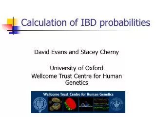
Calculation of IBD probabilities David Evans University of Oxford Wellcome Trust Centre for Human Genetics
This Session … • Identity by Descent (IBD) vs Identity by state (IBS) • Why is IBD important? • Calculating IBD probabilities • Lander-Green Algorithm (MERLIN) • Single locus probabilities • Hidden Markov Model => Multipoint IBD • Other ways of calculating IBD status • Elston-Stewart Algorithm • MCMC approaches • MERLIN • Practical Example • IBD determination • Information content mapping • SNPs vs micro-satellite markers?
Identity By Descent (IBD) 1 2 1 3 1 2 3 4 2 1 1 3 1 4 1 3 Identical by Descent Identical by state only Two alleles are IBD if they are descended from the same ancestral allele
Example: IBD in Siblings Consider a mating between mother AB x father CD: IBD 0 : 1 : 2 = 25% : 50% : 25%
Why is IBD Sharing Important? • Affected relatives not only share disease alleles IBD, but also tend to share marker alleles close to the disease locus IBD more often than chance • IBD sharing forms the basis of non-parametric linkage statistics 1/2 3/4 3/4 1/3 2/4 1/4 4/4 1/4 4/4
A1 Q1 Non-recombinant Parental genotypes (many, 1 – θ) A2 Q2 A1 Q2 Recombinant genotypes (few, θ) Q1 A2 Cosegregation => Linkage Parental genotype A1 Q1 A2 Q2 Alleles close together on the same chromosome tend to stay together in meiosis; therefore they tend be co-transmitted.
Segregating Chromosomes MARKER DISEASE GENE
Marker Shared Among Affecteds 1/2 3/4 3/4 1/3 2/4 1/4 4/4 1/4 4/4 Genotypes for a marker with alleles {1,2,3,4}
Linkage between QTL and marker QTL Marker IBD 0 IBD 1 IBD 2
/ / 1 2 1 2 IBD=0 / 1 1 / 2 2 IBD can be trivial…
/ / / / 1 2 1 2 1 2 1 2 IBD=2 / / / / 1 1 1 1 2 2 2 2 Two Other Simple Cases…
/ / 1 2 2 2 IBD=1 (50% chance) IBD=2 (50% chance) / / 1 2 1 2 A little more complicated…
IBD=? / / 1 1 1 1 And even more complicated…
= P(IBD i , G ) = = P ( IBD i | G ) P ( G ) = = P ( IBD i ) P ( G | IBD i ) = P ( G ) = = P ( IBD i ) P ( G | IBD i ) = å = = P ( IBD j ) P ( G | IBD j ) j=0,1,2 Bayes Theorem for IBD Probabilities
/ / 1 1 1 1 Worked Example = p 0 . 5 1 = = P ( G | IBD 0 ) = = P ( G | IBD 1 ) = = P ( G | IBD 2 ) = P ( G ) = = P ( IBD 0 | G ) = = P ( IBD 1 | G ) = = P ( IBD 2 | G )
/ / 1 1 1 1 Worked Example
For ANY PEDIGREE the inheritance pattern at any point in the genome can be completely described by a binary inheritance vector of length 2n: v(x) = (p1, m1, p2, m2, …,pn,mn) whose coordinates describe the outcome of the paternal and maternal meioses giving rise to the n non-founders in the pedigree pi (mi) is 0 if the grandpaternal allele transmitted pi (mi) is 1 if the grandmaternal allele is transmitted / / a b c d v(x) = [0,0,1,1] / / a c b d
Inheritance Vector In practice, it is not possible to determine the true inheritance vector at every point in the genome, rather we represent partial information as a probability distribution of the possible inheritance vectors Inheritance vector Prior Posterior ------------------------------------------------------------------- 0000 1/16 1/8 0001 1/16 1/8 0010 1/16 0 0011 1/16 0 0100 1/16 1/8 0101 1/16 1/8 0110 1/16 0 0111 1/16 0 1000 1/16 1/8 1001 1/16 1/8 1010 1/16 0 1011 1/16 0 1100 1/16 1/8 1101 1/16 1/8 1110 1/16 0 1111 1/16 0 a b a c 1 2 p1 m1 a c b b 3 4 p2 m2 a b 5
Computer Representation • At each marker location ℓ • Define inheritance vector vℓ • Meiotic outcomes specified in index bit • Likelihood for each gene flow pattern • Conditional on observed genotypes at location ℓ • 22n elements !!! 0000 0001 0010 0011 0100 0101 0110 0111 1000 1001 1010 1011 1100 1101 1110 1111 L L L L L L L L L L L L L L L L
Multipoint IBD • IBD status may not be able to be ascertained with certainty because e.g. the mating is not informative, parental information is not available • IBD information at uninformative loci can be made more precise by examining nearby linked loci
Multipoint IBD / / a b c d / / 1 1 1 2 / / IBD = 0 a c b d IBD = 0 or IBD =1? / / 1 1 1 2
Complexity of the Problemin Larger Pedigrees • For each person • 2n meioses in pedigree with n non-founders • Each meiosis has 2 possible outcomes • Therefore 22npossibilities for each locus • For each genetic locus • One location for each of m genetic markers • Distinct, non-independent meiotic outcomes • Up to 4nm distinct outcomes!!!
Example: Sib-pair Genotyped at 10 Markers P(G | 0000) (1 – θ)4 Inheritance vector 0000 0001 0010 … 1111 1 2 3 4 … m = 10 Marker (22xn)m = (22 x 2)10 =~ 1012 possible paths !!!
P(IBD) = 2 at Marker Three IBD Inheritance vector 0000 (2) (1) 0001 (1) 0010 … (2) 1111 1 2 3 4 … m = 10 Marker (L[0000] + L[0101] + L[1010] + L[1111] ) / L[ALL]
P(IBD) = 2 at arbitrary position on the chromosome Inheritance vector 0000 0001 0010 … 1111 1 2 3 4 … m = 10 Marker (L[0000] + L[0101] + L[1010] + L[1111] ) / L[ALL]
Lander-Green Algorithm • The inheritance vector at a locus is conditionally independent of the inheritance vectors at all preceding loci given the inheritance vector at the immediately preceding locus (“Hidden Markov chain”) • The conditional probability of an inheritance vector vi+1 at locus i+1, given the inheritance vector vi at locus i is θij(1-θi)2n-j where θ is the recombination fraction and j is the number of changes in elements of the inheritance vector Example: Locus 1 Locus 2 [0000] [0001] Conditional probability = (1 – θ)3θ
Lander-Green Algorithm Inheritance vector 0000 0001 0010 … 1111 1 2 3 4 … m = 10 Marker M(22n)2 = 10 x 162 = 2560 calculations
0000 0001 0010 … 1111 1 2 3 … m Total Likelihood = 1’Q1T1Q2T2…Tm-1Qm1 P(G|[0000]) 0 0 0 (1-θ)4 (1-θ)3θ … θ4 0 P(G|[0001]) 0 0 (1-θ)4 (1-θ)3θ … (1-θ)θ3 Qi = Ti = 0 0 … 0 … … … … 0 0 0 P(G|[1111]) θ4 (1-θ)θ3 … (1-θ)4 22n x 22n diagonal matrix of single locus probabilities at locus i 22n x 22n matrix of transitional probabilities between locus i and locus i+1 ~m(22n)2 operations = 2560 for this case !!!
Further speedups… • Trees summarize redundant information • Portions of vector that are repeated • Portions of vector that are constant or zero • Speeding up convolution • Use sparse-matrix by vector multiplication • Use symmetries in divide and conquer algorithm (Idury & Elston, 1997)
Lander-Green Algorithm Summary • Factorize likelihood by marker • Complexity m·en • Strengths • Large number of markers • Relatively small pedigrees
Elston-Stewart Algorithm • Factorize likelihood by individual • Complexity n·em • Small number of markers • Large pedigrees • With little inbreeding • VITESSE, FASTLINK etc
Other methods • Number of MCMC methods proposed • ~Linear on # markers • ~Linear on # people • Hard to guarantee convergence on very large datasets • Many widely separated local minima • E.g. SIMWALK
Linkage Analysis NPL and K&C LOD Variance Components Haplotypes Most likely Sampling All IBD and info content Error Detection Most SNP typing errors are Mendelian consistent Recombination No. of recombinants per family per interval can be controlled Simulation Capabilities
Reference FAQ Source Binaries Tutorial Linkage Haplotyping Simulation Error detection IBD calculation MERLIN Website www.sph.umich.edu/csg/abecasis/Merlin
Input Files • Pedigree File • Relationships • Genotype data • Phenotype data • Data File • Describes contents of pedigree file • Map File • Records location of genetic markers
Example Pedigree File <contents of example.ped> 1 1 0 0 1 1 x 3 3 x x 1 2 0 0 2 1 x 4 4 x x 1 3 0 0 1 1 x 1 2 x x 1 4 1 2 2 1 x 4 3 x x 1 5 3 4 2 2 1.234 1 3 2 2 1 6 3 4 1 2 4.321 2 4 2 2 <end of example.ped> Encodes family relationships, marker and phenotype information
Example Data File <contents of example.dat> T some_trait_of_interest M some_marker M another_marker <end of example.dat> Provides information necessary to decode pedigree file
Example Map File <contents of example.map> CHROMOSOME MARKER POSITION 2 D2S160 160.0 2 D2S308 165.0 … <end of example.map> Indicates location of individual markers, necessary to derive recombination fractions between them
/ / 1 1 1 1 Worked Example = p 0 . 5 1 1 = = P ( IBD 0 | G ) 9 4 = = P ( IBD 1 | G ) 9 4 = = P ( IBD 2 | G ) 9 merlin –d example.dat –p example.ped –m example.map --ibd
Application: Information Content Mapping • Information content: Provides a measure of how well a marker set approaches the goal of completely determining the inheritance outcome • Based on concept of entropy • E = -ΣPilog2Pi where Pi is probability of the ith outcome • IE(x) = 1 – E(x)/E0 • Always lies between 0 and 1 • Does not depend on test for linkage • Scales linearly with power
Application: Information Content Mapping • Simulations • ABI (1 micro-satellite per 10cM) • deCODE (1 microsatellite per 3cM) • Illumina (1 SNP per 0.5cM) • Affymetrix (1 SNP per 0.2 cM) • Which panel performs best in terms of extracting marker information? merlin –d file.dat –p file.ped –m file.map --information
SNP microsat 0.2 cM 3 cM 0.5 cM 10 cM SNPs vs Microsatellites 1.0 SNPs + parents 0.9 microsat + parents 0.8 0.7 0.6 Information Content 0.5 0.4 0.3 Densities 0.2 0.1 0.0 0 10 20 30 40 50 60 70 80 90 100 Position (cM)