Download
1 / 46
460 likes | 554 Views
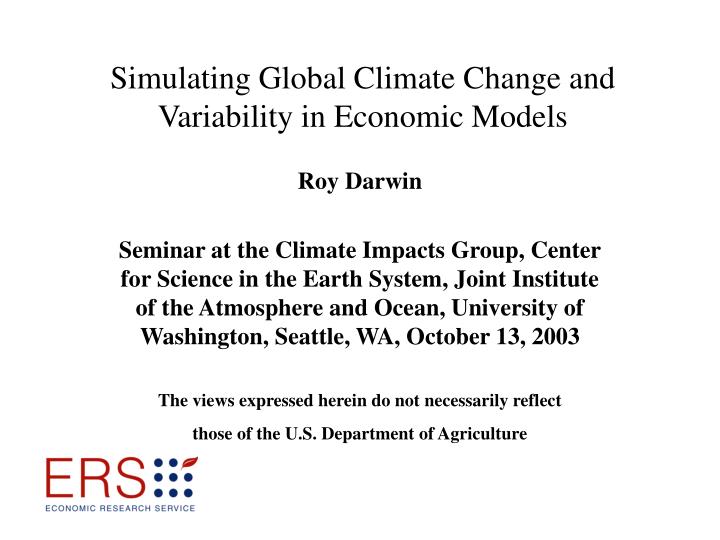
Simulating Global Climate Change and Variability in Economic Models. Roy Darwin Seminar at the Climate Impacts Group, Center for Science in the Earth System, Joint Institute of the Atmosphere and Ocean, University of Washington, Seattle, WA, October 13, 2003

E N D
Simulating Global Climate Change and Variability in Economic Models Roy Darwin Seminar at the Climate Impacts Group, Center for Science in the Earth System, Joint Institute of the Atmosphere and Ocean, University of Washington, Seattle, WA, October 13, 2003 The views expressed herein do not necessarily reflect those of the U.S. Department of Agriculture
Outline • Future Agricultural Resources Model • Climate Variability • Inter-Annual Variability
FARM’s Environmental Component Land Cover Climate Growing Season Water Runoff Land Characteristics Water Supply FARM’s Economic Component
FARM’s Economic Component FARM’s Environmental Component Land Water Labor Capital Production Possibilities Other Regions Payments Supply/Demand Population Foreign Region1 Production Income Trade Payments Supply/Demand Foreign Region n Consumer Preferences
Topics Analyzed with FARM • Impacts of greenhouse gas emissions on agriculture and forestry • Costs of sea level rise • Effects of trade deregulation and population growth on tropical forests • Costs of protecting global ecosystem diversity • Impacts of technological advance in agriculture on land use
Database Components • Land cover • Agro-ecological zones • Production • Production distribution
Land Cover Component • The land-cover component organizes data on land cover characteristics • The main data source is a 1-km resolution global land cover characteristics database • These data are organized by 0.5 grid and second order political unit • The original category codes were normalized, disaggregated, and reaggregated into 10 general land-cover categories
Percent Grassland Derived from: U.S. Geological Survey. EROS Data Center. Global Land Cover Characteristics Data Base Version 2.0. , 2001.
Percent Tundra Derived from: U.S. Geological Survey. EROS Data Center. Global Land Cover Characteristics Data Base Version 2.0. , 2001.
Percent Coniferous Forestland Derived from: U.S. Geological Survey. EROS Data Center. Global Land Cover Characteristics Data Base Version 2.0. , 2001.
Percent Nonconiferous Forestland Derived from: U.S. Geological Survey. EROS Data Center. Global Land Cover Characteristics Data Base Version 2.0. , 2001.
Percent Mixed Forestland Derived from: U.S. Geological Survey. EROS Data Center. Global Land Cover Characteristics Data Base Version 2.0. , 2001.
Percent Scattered Trees Derived from: U.S. Geological Survey. EROS Data Center. Global Land Cover Characteristics Data Base Version 2.0. , 2001.
Percent Shrubland Derived from: U.S. Geological Survey. EROS Data Center. Global Land Cover Characteristics Data Base Version 2.0. , 2001.
Percent Built-Up Land Derived from: U.S. Geological Survey. EROS Data Center. Global Land Cover Characteristics Data Base Version 2.0. , 2001.
Percent Other Land Derived from: U.S. Geological Survey. EROS Data Center. Global Land Cover Characteristics Data Base Version 2.0. , 2001.
Percent Cropland in 1997 Derived from: U.S. Geological Survey. EROS Data Center. Global Land Cover Characteristics Data Base Version 2.0. , 2001; Food and Agriculture Organization of the United Nations. FAOSTAT Agriculture Data. 2001; Döll, P. and S. Siebert. A digital global map of irrigated areas. 2000; Siebert, S. and P. Döll. A digital global map of irrigated areas—An update for Latin America and Europe. 2001.
Percent Irrigated Land in 1997 Derived from: Döll, P. and S. Siebert. A digital global map of irrigated areas. 2000; Siebert, S. and P. Döll. A digital global map of irrigated areas—An update for Latin America and Europe. 2001; U.S. Geological Survey. EROS Data Center. Global Land Cover Characteristics Data Base Version 2.0. 2001; Food and Agriculture Organization of the United Nations. FAOSTAT Agriculture Data. 2001.
Agro-Ecological Zone Component • Agro-ecological zones (AEZs) replace land classes in the current version of FARM • The AEZ component constructs AEZs based on length of growing season and thermal regime • Growing season and thermal regime are calculated from meteorological data with a soil temperature and moisture algorithm • The meteorological data are monthly temperature and precipitation at 0.5-degree grid, 1901-1998
Rainfed Agro-Ecological Zones in 1997 Derived from: University of East Anglia. Climate Research Unit. CRU05 0.5 Degree 1901-1995 Monthly Climate Time-Series. East Anglia, Great Britain.
Rainfed Thermal Regimes in 1997 Derived from: University of East Anglia. Climate Research Unit. CRU05 0.5 Degree 1901-1995 Monthly Climate Time-Series. East Anglia, Great Britain.
Production Component • The production component organizes price and quantity data for agricultural and forestry commodities • It tracks production of 173 crops by country • It tracks 37 primary livestock commodities • It tracks 6 categories of timber products • It also tracks 18 categories of live animals
Production Distribution Component • The production distribution component links production to land covers by AEZ • Commodities are distributed to appropriate land covers • Average production for each AEZ in the appropriate land cover is estimated with regression analysis • Commodities are distributed by AEZ and calibrated to official levels
Wheat Production in 1997 (mt/1000ha land) Interpolated from country or state level data
Paddy Rice Production in 1997 (mt/1000ha land) Interpolated from country or state level data
Distributing Livestock and Forest Products • Many grasslands or forestlands do not provide livestock or forest products because people do not live there • A particular livestock animal, livestock commodity, or forest product may be associated with more than one land cover • Consistency between live animals and livestock commodities must be maintained
Population Density in 1998 (no/1000ha land) Derived form Oak Ridge National Laboratory. LandScan Global Population 1998 Database, Oak Ridge, Tennessee.
Cattle Inventory in 1997 (head/1000 ha land) Interpolated from country and state level data
Beef, Veal, and Cattle Hide Production in 1997 (mt/1000ha land) Interpolated from country and state level data
Cow Milk Production in 1997 (mt/1000ha land) Interpolated from country and state level data
Conifer Sawlog Production in 1997 (m3/1000ha land) Interpolated from country and U.S. regional level data
Nonconifer Sawlog Production in 1997 (m3/1000ha land) Interpolated from country and U.S. regional level data
%CQ = -0.223 T, adjR2 = 0.832 (-6.656)
%CP = 0.577 T, adjR2 = 0.930 (9.809)
%W = -0.015 T, adjR2 = 0.541 (-3.431)
%W = 0.018 T, adjR2 = 0.644 (4.225)
%W = -0.157 T, adjR2 = 0.935 (-9.694)
Estimating Impacts of Meteorological Phenomena on Length of Growing Seasons in the 20th Century • Yi = 0 + 1T + 2ENSOj + 3ENSOj*Dj + whereYiis a vector of irrigated or rainfed growing season lengths, T is a trend vector equal to (1,96), ENSOj is either a SOI or CTI vector, Dj is a dummy variable (= 0 when ENSOj 0, but = 1 when ENSOj 0), and is a vector of error terms with a finite variance
Estimated Average Change in Length of Rainfed Growing Season, 1902-1997: Derived from Regression Models Using the CTI to Capture ENSO Cycles: Days and Confidence
Estimated Average Impact of El Niño on Length of Rainfed Growing Season, 1902-1997: Derived from Regression Models Using the CTI to Capture ENSO Cycles: Days and Confidence
Estimated Average Impact of La Niña on Length of Rainfed Growing Season, 1902-1997: Derived from Regression Models Using the CTI to Capture ENSO Cycles: Days and Confidence
Current Cropland in Low-Income Countries Affected by Climate-Induced Changes in Growing Season Estimated with results from regression models with the Cold Tongue Index for the El Niño/Southern Oscillation cycle.
Impact of Climate Change on Cropland Growing Seasons in Selected Low-Income Countries, 1902-1997 Estimated with results from regression models with the Cold Tongue Index for the El Niño/Southern Oscillation cycle.
Food Distribution Gap in Various Low-Income Countries Projected for 2012 (kg grain/person) Estimated with ERS’s Food Security Assessment model
Estimated Contribution of Climate-Induced Changes in Average Growing Season to 2012 Projections of Food Distribution Gaps in Selected Low Income Countries (percent) Estimated with ERS’s Food Security Assessment model