Download
1 / 13
130 likes | 342 Views
Transient Thermal Problems. Jake Blanchard Spring 2008. Transient Analyses. So far, all the problems we’ve discussed in this class have all been steady state problems. ANSYS is capable of doing a wide variety of transient problems. We’ll explore this with a thermal problem. Sample Problem.

E N D
Transient Thermal Problems Jake Blanchard Spring 2008
Transient Analyses • So far, all the problems we’ve discussed in this class have all been steady state problems. • ANSYS is capable of doing a wide variety of transient problems. • We’ll explore this with a thermal problem.
Sample Problem h=1000 W/m2-K Tb=50 C • Channel is 3 cm in diameter • k=80 W/m-K • =8000 kg/m3 • cp=500 J/kg-K • Do steady state analysis now. 3 cm 9 cm 9 cm q=104 W/m2
Transient Problem • The question is, if we start the body at a uniform temperature of 50 C, how long does it take to reach steady state?
Steps • Define time dependent loads (in load steps) • Set analysis parameters (time at end of load step, number of time steps, etc.) • Solve • Look at results
Load History for Sample Problem • Load Step 1: Ramp up flux • Load Step 2: Flux is steady • Load Step 3: Turn off flux and let structure cool back to 50 C q (W/m-K) 104 1000 5000 Time (s)
Setting Up a Time Step • Set parameters for end of step (mostly loads) • Set time for end of step • Set number of time steps • Save settings
First Load Step • Set analysis type to transient (Solution/Analysis Type/New Analysis) • Set time at end of step to 1,000 seconds (Solution/Analysis Type/Sol’n Controls) • Set initial temperatures (Define Loads/Apply/Initial Condition/Define) • Set convection and heat flux loads (heat flux is value at end of step) • Choose Ramped or Stepped • Only load is convection
Post Processing • Options • Read a load step, then do usual postprocessing (contour plots, etc.) • Use time history processor to plot a particular value as a function of time • Animate contours (try PlotCtrls/Style/Contours/Uniform Contours)
Load Step 2 • Only change is time at end of step (loads don’t change) • Solve
Load Step 3 • Delete heat flux • Set time at end (try 10,000 seconds) • Solve