Download
1 / 37
380 likes | 700 Views
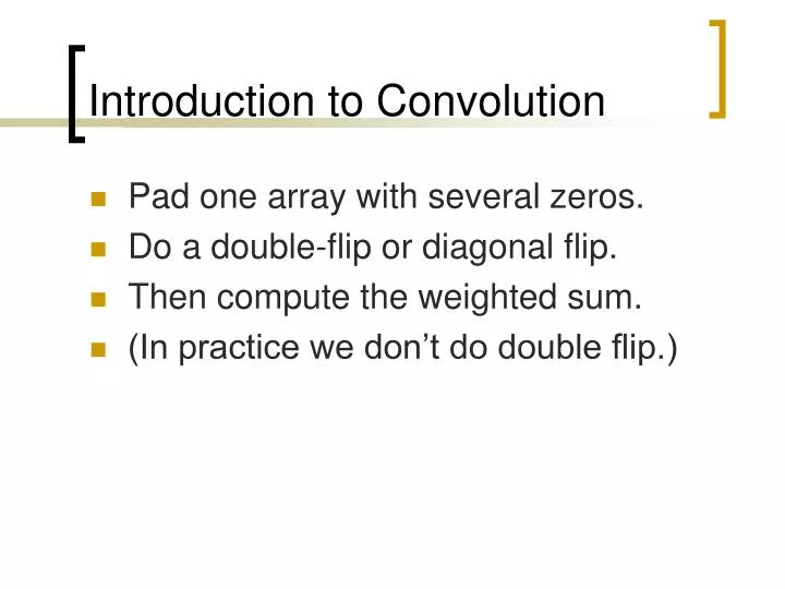
Introduction to Convolution. Pad one array with several zeros. Do a double-flip or diagonal flip. Then compute the weighted sum. (In practice we don’t do double flip.). Convolution: Step One Padding an array with zeros. [ ]. -1 +1 -2 +2. 0 0 0 0 0 0 0 0 0 0 0 0

E N D
Introduction to Convolution • Pad one array with several zeros. • Do a double-flip or diagonal flip. • Then compute the weighted sum. • (In practice we don’t do double flip.)
Convolution: Step One Padding an array with zeros [ ] -1 +1 -2 +2 0 0 0 0 0 0 0 0 0 0 0 0 0 0 -1 +1 0 0 0 0 -2 +2 0 0 0 0 0 0 0 0 0 0 0 0 0 0
Convolution :Double Flip of the “Reflected Function” [ ] 0 2 1 3 [ ] 1 3 0 2 [ ] 3 1 2 0
Computing Weighted Sum: Step 3 0 0 0 0 0 0 0 0 0 0 0 0 0 0 -1 +1 0 0 0 0 -2 +2 0 0 0 0 0 0 0 0 0 0 0 0 0 0 [ ] 3 1 2 0 3*0 + 1*0 + 2*0 + 0*0 This calculates the weighted sum. The weights Summing these numbers [] • Note: each weighted sum results in • one number. • This number gets placed in the output • array in the position that the inputs came • from. 0
The previous slide…. • Was an example of a one-location convolution. • If we move the location of the numbers being summed, we have scanning convolution. • The next slides show the scanning convolution.
Computing Weighted Sum: Step 3 0 0 0 0 0 0 0 0 0 0 0 0 0 0 -1 +1 0 0 0 0 -2 +2 0 0 0 0 0 0 0 0 0 0 0 0 0 0 [ ] 3 1 2 0 3*0 + 1*0 + 2*0 + 0*0 This calculates the next weighted sum. The weights • This number gets placed in the output • array in the NEXT position. Summing these numbers [] 0 0
Computing Weighted Sum: Step 3 0 0 0 0 0 0 0 0 0 0 0 0 0 0 -1 +1 0 0 0 0 -2 +2 0 0 0 0 0 0 0 0 0 0 0 0 0 0 [ ] 3 1 2 0 3*2 + 1*0 + 2*0 + 0*0 This calculates the next weighted sum. The weights • This number gets placed in the output • array in the NEXT position. Summing these numbers [] 0 0 6
Computing Weighted Sum • Two arrays of four numbers each • One is the image, the other is the weights. • The result is the weighted sum. [] [] = [] -1 +1 -2 +2 * 0 2 1 3 0 -2 +2 -1 -6 +7 -2 -4 +6 (weights) (image) (weighted sum)
Edge Detection • Create the algorithm in pseudocode: while row not ended // keep scanning until end of row select the next A and B pair diff = B – A //formula to show math if abs(diff) > Threshold //(THR) mark as edge Above is a simple solution to detecting the differences in pixel values that are side by side.
Link here to Sliding Box • To sliding box
Edge Detection: One-location Convolution • diff = B – A is the same as: A B -1 +1 * Box 2 (“weights”) Box 1 Convolution symbol Place box 2 on top of box 1, multiply. -1 * A and +1 * B Result is –A + B which is the same as B – A
Edge Detection • Create the algorithm in pseudocode: while row not ended // keep scanning until end of row select the next A and B pair diff = //formula to show math if abs(diff) > Threshold //(THR) mark as edge * A B -1 +1 Above is a simple solution to detecting the differences in pixel values that are side by side.
Edge Detection:Pixel Values Become Gradient Values • 2 pixel values are derived from two measurements • Horizontal • Vertical A B -1 +1 * Note: A,B pixel pair will be moved over whole image to get different answers at different positions on the image A -1 * B +1
The Resulting Vectors • Two values are then considered vectors • The vector is a pair of numbers: • [Horizontal answer, Vertical answer] • This pair of numbers can also be represented by magnitude and direction
Edge Detection:Vectors • The magnitude of a vector is the square root of the numbers from the convolution √ (a)² + (b)² a is horizontal answer b is vertical answer
Edge Detection:Deriving Gradient, the Math • The gradient is made up of two quantities: • The derivative of I with respect to x • The derivative of I with respect to y ∂ = derivative symbol ∆ = is defined as = I = [ ] ∂ I∂ I ∂x , ∂ y ∆ ||I|| So the gradient of I is the magnitude of the gradient. Arrived at mathematically by the “simple” Roberts algorithm. The Sobel method takes the average Of 4 pixels to smooth (applying a smoothing feature before finding edges. √ ) ( ) ( ∂ I 2 ∂ I 2 ∂x + ∂ y
Effect of Thresholding Threshold Bar
Thresholding the Gradient Magnitude • Whatever the gradient magnitude is, for example, in the previous slide, with two blips, we picked a threshold number to decide if a pixel is to be labeled an edge or not. • The next three slides will shows one example of different thresholding limits.
Magnitude Output with a high bar (threshold number) Edges have thinned out, but horses head and other parts of the pawn have disappeared. We can hardly see the edges on the bottom two pieces.
Magnitude Formula in the c Code /* Applying the Magnitude formula in the code*/ maxival = 0; for (i=mr;i<256-mr;i++) { for (j=mr;j<256-mr;j++) { ival[i][j]=sqrt((double)((outpicx[i][j]*outpicx[i][j]) + (outpicy[i][j]*outpicy[i][j])); if (ival[i][j] > maxival) maxival = ival[i][j]; } }
Edge Detection Graph shows one line of pixel values from an image. Where did this graph come from?
Smoothening before Difference Smoothening in this case was obtained by averaging two neighboring pixels.
Edge Detection Graph shows one line of pixel values from an image. Where did this graph come from?
Smoothening rationale • Smoothening: We need to smoothen before we apply the derivative convolution. • We mean read an image, smoothen it, and then take it’s gradient. • Then apply the threshold.
The Four Ones • The way we will take an average of four neighboring pixels is to convolve the pixels with [] ¼ ¼ ¼ ¼ Convolving with this is equal to a + b + c + d divided by 4. (Where a,b,c,d are the four neighboring pixels.)
Four Ones, cont. [] [] ¼ ¼ ¼ ¼ 1 1 1 1 Can also be written as: 1/4 Meaning now, to get the complete answer, we should compute: ( ) [] [ ] [ ] 1 1 1 1 -1 +1 -1 +1 * * Image 1/4
Four Ones, cont. ( ) [] [ ] [ ] 1 1 1 1 -1 +1 -1 +1 * * Image 1/4 By the associative property of convolution we get this next step. [ ] [ ] ( ) [ ] 1 1 1 1 -1 +1 -1 +1 * * Image 1/4 We do this to call the convolution code only once, which precomputes The quantities in the parentheses.
Four Ones, cont. ( ) [ ] 1 1 1 1 [ ] -1 +1 -1 +1 * As we did in the convolution slide: We combine this to get: This table is a result of doing a scanning convolution.
The magnitude of the gradient is then calculated using the formula which we have seen before:
Sobel Algorithm…another way to look at it. • The Sobel algorithm uses a smoothener to lessen the effect of noise present in most images. This combined with the Roberts produces these two – 3X3 convolution masks. Gx Gy
Step 1 – use small image with only black (pixel value = 0) and white (pixel value = 255) 20 X 20 pixel image of black box on square white background Pixel values for above image
X mask values Step 2 – Apply Sobel masks to the image, first the x and then the y. Y mask values
X mask Step 3 – Find the Magnitudes using the formula c = sqrt(X2 + Y2) Magnitudes Y mask
Step 4 – Apply threshold, say 150, to the combined image to produce final image. Before threshold After threshold of 150 These are the edges it found